Intercept and preload
A measured nonzero intercept can indicate sensor offset, fixture drag, adhesion, or preload. Do not force it to zero merely to match the calculator.
Physics and mechanics
Generate an exact static-limit and kinetic-friction data series across increasing normal loads, with per-record work for plotting and reconciliation.
FRICTION DATA SERIES
A friction graph is only as defensible as the values and model behind each point. This page creates a compact normal-load series, calculates static and kinetic lines independently, and preserves the exact table used by a later plot.
FRICTION DATA SERIES
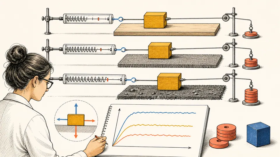
The table is the evidence. Any visual graph must use these exact ordered records and identify them as model outputs rather than measurements.
| Record | Normal force N | Static limit N | Kinetic force N | Kinetic work J |
|---|
DETAILED CALCULATION PROCESS
Fs,max(Ni) = mus Ni; Fk(Ni) = muk Ni; Wi = Fk(Ni) d; Ni = N0 + i DeltaN
Generate ordered normal-load values, multiply each by the two declared coefficients, and attach kinetic work over the common sliding distance to every record.
| Symbol | Meaning | Unit | Default-page basis |
|---|---|---|---|
| Ni | Normal force at record i | N | start + i × step |
| mus | Static friction coefficient | dimensionless | entered static slope |
| muk | Kinetic friction coefficient | dimensionless | entered kinetic slope |
| Fs,max | Maximum static-friction limit | N | mus × Ni |
| Fk | Kinetic friction force | N | muk × Ni |
| Wi | Kinetic work for record i | J | Fk × distance |
RESULT INTERPRETATION
The static-limit and kinetic-force columns are straight lines because each is generated by a constant coefficient multiplied by normal force. Their slopes are the entered coefficients and their intercepts are fixed at zero. Smoothness is guaranteed by the formula and cannot validate a material claim.
The final force values describe only the largest generated normal-load record. Summed kinetic work adds the hypothetical work attached to every row; it should not be interpreted as one physical cycle unless those records truly occur in sequence. Export the ordered table when comparing with measurements.
DECISION BOUNDARY
The table is the evidence. Any visual graph must use these exact ordered records and identify them as model outputs rather than measurements.
A measured nonzero intercept can indicate sensor offset, fixture drag, adhesion, or preload. Do not force it to zero merely to match the calculator.
SENSITIVITY AND STRESS TESTING
Curvature or changing residuals can show that one constant coefficient is not valid across the selected load range.
Preserve acquisition order, calibration, repeated readings, and uncertainty. A fitted line without those records can hide drift, hysteresis, or surface evolution.
HOW TO USE THIS CALCULATOR
SUBJECT FOUNDATIONS
MODEL BOUNDARY
Generate ordered normal-load values, multiply each by the two declared coefficients, and attach kinetic work over the common sliding distance to every record.
DECISION DEPTH
A fitted measured line that does not pass through zero can reflect sensor offset, preload, adhesion, or fixture drag. This ideal series forces zero intercept.
Real polymers, soft contacts, lubricated interfaces, and rough surfaces may not remain linear across the selected range.
A smooth line is guaranteed by the formula. Validation requires independent measurements and residual analysis.
REAL USE CASES
An instructor generates expected static and kinetic values, then asks students to compare measured records and discuss residuals.
An engineer uses the final static limit to screen whether the chosen sensor can capture breakaway force without saturation.
TERMS USED ON THIS PAGE
EVIDENCE TO RETAIN
Keep coefficient sources, material condition, load range, record order, step size, sliding distance, generated unrounded values, any plotted version, measurement uncertainty, sensor calibration, and a clear model-versus-measurement label.
LIMITS AND EXCLUSIONS
RELIABLE SOURCES
QUESTIONS SPECIFIC TO THIS CALCULATION
This page uses the common dry-contact Coulomb ordering. Other regimes require a different model and evidence.
No. Every point is calculated from the entered coefficients and loads.
It connects each kinetic-force record to an energy consequence over the declared distance.
Use external analysis software for larger series; the page limits records to keep the audit table readable.
No fit is needed because the equation defines the line. Regression is meaningful when comparing independent measurements.
Check coefficient domain, load effects, sensor offsets, surface change, and whether a non-Coulomb model is needed.
The page generates an ideal Coulomb series with zero intercept. Estimating an intercept belongs to regression on independent measured data.
Only if the listed loads and distances actually represent sequential events in the campaign. Otherwise it is a worksheet total across separate hypothetical rows.
Retain raw values and uncertainty, fit an appropriate model, inspect residuals and order effects, and label the calculated line separately from observations.
Load order may match an experimental sequence or operating ramp. Sorting can hide drift, hysteresis, conditioning, or a direction-dependent effect in later comparisons.
IMPORTANT BOUNDARY
This calculator generates idealized Coulomb-friction records for education and preliminary planning. It does not certify materials, sensors, machinery, or safety factors.