Bayes’ Theorem: How Evidence Changes a Probability

A test turns positive. A message contains a suspicious word. A sensor reports an anomaly. The tempting question is, “How likely is the cause?” The number a test-maker usually gives—how often the signal appears when the cause is present—answers a different question. Bayes’ theorem is the conversion rule that keeps those directions separate.

For events A and B, with P(B) > 0P(A | B) = P(B | A) P(A) / P(B)

Posterior = likelihood × prior, divided by the total probability of the evidence.

An analyst operates a navy balance apparatus where one orange evidence ball changes a vessel labeled prior and releases teal probability tiles — Evidence changes a starting probability; it does not make the starting probability disappear. The update only means what its population and evidence model mean.

The four parts of an update

P(A)Prior

The chance of the target event before seeing B.

P(B | A)Likelihood

How compatible the evidence is with A.

P(B)Evidence total

Every modeled route by which B could occur.

P(A | B)Posterior

The revised chance of A after B is known.

All four quantities are dimensionless probabilities from 0 to 1. That makes the unit check simple: a product of two probabilities, divided by one probability, is still dimensionless. The catch is semantic, not mechanical. You must state what A, B, the population, and the time window are before inserting numbers.

For competing hypotheses A₁, …, Aₙ that are mutually exclusive and exhaustive, the denominator becomes a weighted total:

P(A_k | B) = P(B | A_k)P(A_k) / Σ_iP(B | A_i)P(A_i)

The denominator is the normalizer. Leave out a plausible route to B and the resulting “posterior” is not a probability across the intended set.

Why the formula is true

Bayes’ theorem is not an extra assumption about independence. It follows from writing the same joint event in two valid orders. The National Institute of Standards and Technology presents this same joint-probability derivation in its Bayesian experiment-design material.

1. Condition on BP(A ∩ B) = P(A | B)P(B)

2. Condition on AP(A ∩ B) = P(B | A)P(A)

3. Equate and divideP(A | B) = P(B | A)P(A) / P(B)

The useful inverse forms are just as direct: P(B | A) = P(A | B)P(B)/P(A) and P(A) = P(A | B)P(B)/P(B | A), when the relevant denominators are non-zero. In practice, however, the denominator is usually the harder part: it requires thinking about alternatives rather than only the target case.

Worked example: a positive screening result

This is a hypothetical arithmetic model, not medical advice or a performance claim about any assay. Let D mean that a condition is present and + a positive result. In a specified screened population, suppose prevalence is P(D) = 0.0100, sensitivity is P(+ | D) = 0.950, and specificity is P(− | not D) = 0.900. The false-positive rate is therefore P(+ | not D) = 0.100.

True-positive route(0.950)(0.0100) = 0.00950

False-positive route(0.100)(0.9900) = 0.0990

Posterior0.00950 / (0.00950 + 0.0990) = 0.0875576

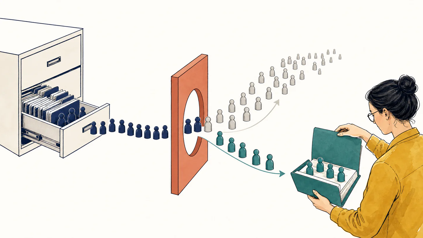
The model gives P(D | +) = 8.76%, not 95%. A frequency check makes the denominator visible: among 10,000 people, 100 have the condition and yield 95 true positives; 9,900 do not and yield 990 false positives. So 95 of 1,085 positive results are true positives: 95/1,085 = 0.0875576. The CDC’s screening guidance calls this positive predictive value and emphasizes its dependence on prevalence.

Patient tokens pass through an orange test gate, with many gray tokens diverting away and a smaller teal group collected by a clinician — A signal can be common among true cases and still produce many false positives when the target condition is rare in the screened population.

Worked example: a spam signal

Now let S mean “message is spam” and W mean “message contains a particular signal.” Suppose P(S)=0.20, P(W | S)=0.80, and P(W | not S)=0.10. Here the same reversal gives:

Spam-and-signal route(0.80)(0.20) = 0.160

Legitimate-and-signal route(0.10)(0.80) = 0.080

Posterior0.160 / (0.160 + 0.080) = 2/3 = 66.7%

In 1,000 messages, that means 160 signal-bearing spam messages and 80 signal-bearing legitimate messages: 160/(160+80)=2/3. The likelihood is 80%, but the posterior is 66.7%, because legitimate messages can carry the signal too.

Mistakes that change the answer

Reverse the conditional

P(+ | D) is sensitivity; P(D | +) is a posterior. They can be far apart.

Erase the base rate

Using only a test’s sensitivity skips the prior and makes a low-prevalence result look stronger than it is.

Count a clue twice

Bayes does not grant independence. Correlated signals need a joint likelihood, not two multiplications.

Call a posterior a decision

Probability alone does not set an action. Costs, benefits, and follow-up options still matter.

An analyst lifts a lilac cover from an evidence board to reveal two orange clue strings meeting at one shared pin — Two observations may look separate yet arise from one shared cause. Treating them as independent can produce an overconfident update.

What Bayes can and cannot say

Bayes’ theorem returns a probability conditional on the supplied model. It is excellent for stating how a prior and a likelihood fit together, for comparing defined hypotheses, and for exposing which missing number is doing the work. It does not establish causation, repair a biased sample, prove that the chosen hypotheses are complete, or make uncertain sensitivity and specificity exact.

In continuous-parameter work, the analogous expression uses densities: p(θ | y) = p(y | θ)p(θ)/p(y). A density at one exact point is not a probability and may exceed one; probabilities come from integrating over a stated interval. That distinction, plus model calibration and uncertainty in the inputs, matters whenever an update informs a high-stakes decision.

The most responsible Bayes calculation therefore starts with a sentence, not an equation: “In this population, over this time window, for this precisely defined evidence, what alternatives could have produced the observation?” Once that sentence is sound, the arithmetic is usually the easy part.