Why does water speed up in a narrow pipe, while the static pressure usually falls? Why can a Pitot tube infer airspeed from a small pressure difference? Bernoulli’s equation answers both questions by keeping an energy ledger along a streamline.
For an ideal, steady flow of an incompressible, inviscid fluid with no pump or turbine between two points,
p + ½ρv² + ρgz = constantPressure energy, kinetic energy, and gravitational potential energy trade places along one streamline.
The equation is powerful because it is a conservation statement, not a slogan that “fast flow always means low pressure.” The streamline, elevation, fluid model, and pressure reference all matter.
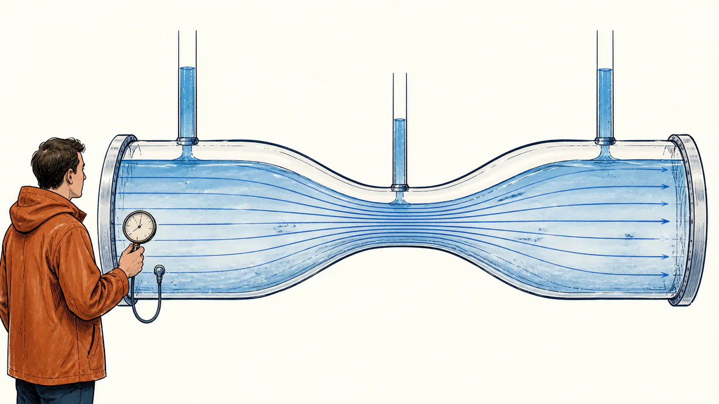
Read the energy ledger before calculating
The pressure-form variables have coherent SI units:
Each term is energy per unit volume:
p → Pa = J/m³½ρv² → (kg/m³)(m²/s²) = J/m³ρgz → (kg/m³)(m/s²)(m) = J/m³The same balance can be divided by ρ into energy per unit mass, or by ρg into head (energy per unit weight):
p/ρ + v²/2 + gz = constantJ/kg, or m²/s².
p/(ρg) + v²/(2g) + z = constantmetres of fluid.
The reference pressure can be gauge or absolute, provided it is used consistently at both points. A gauge pressure of zero at an open free surface is not an absolute vacuum; it means the pressure equals the local atmosphere. BIPM’s SI Brochure provides the unit framework, while OpenStax’s Bernoulli chapter presents the pressure, speed, and height terms. Its pressure-measurement chapter separates gauge from absolute pressure.
Static, dynamic, and stagnation pressure are related but not interchangeable labels. Static pressure is what a pressure tap moving with the fluid would read. Dynamic pressure, q=½ρv², is the kinetic-energy-density term; it is not an additional fluid pressure that exists independently of the flow. Stagnation pressure is the pressure obtained after ideal, lossless deceleration to zero speed. At equal elevation in the incompressible model, p0=p+q. Either static or stagnation pressure can be reported as gauge or absolute, so the full label should say both what physical state is measured and what reference is used.
This vocabulary prevents a common Pitot mistake: adding atmospheric pressure to a gauge reading because the word “total” sounds like “absolute.” The correct operation is to preserve the pressure type and reference separately. For cavitation, density, and gas thermodynamics, use absolute pressure; for a differential-pressure Venturi calculation, a common gauge reference is often convenient.
The datum is equally bookkeeping-friendly. Raising every stated elevation by the same constant adds the same amount to both sides and changes nothing. What matters is the vertical difference between the selected points, not whether the datum is sea level, a bench, or the pipe centerline. Naming that datum in a calculator makes sign errors easier to audit.
Why the three terms trade off
Take a small fluid parcel moving from point 1 to point 2. Pressure forces do work on the parcel as it enters and leaves a control volume. Gravity changes its potential energy, and the parcel’s speed changes its kinetic energy. For steady inviscid flow, there is no viscous dissipation, so the work–energy balance is
p1 − p2½ρ(v2² − v1²)ρg(z2 − z1)p1 + ½ρv1² + ρgz1 = p2 + ½ρv2² + ρgz2The integration assumes a streamline. In an irrotational flow, the constant can be shared across streamlines, but a rotating or strongly three-dimensional flow may have different constants from one streamline to another. Do not silently turn a streamline equation into a whole-tank equation.
Continuity supplies the missing speed
Bernoulli relates pressure and speed, but it does not by itself determine either speed. For steady incompressible flow through a pipe, conservation of mass gives
Q = AvA1v1 = A2v2Volumetric flow rate Q is in m³/s; pipe area A is in m².
For a circular pipe, A=πD²/4, so
v2 = v1(D1/D2)²A diameter ratio must be squared.Halving a diameter makes the area one quarter as large, so the speed becomes four times larger if the same incompressible flow rate passes through. Many wrong Venturi answers come from using D1/D2 instead of its square.
Rearrangements and domain checks
The two-point pressure form can solve for a missing quantity, but every rearrangement keeps the original assumptions. For example,
p2=p1+½ρ(v1²−v2²)+ρg(z1−z2)v2=√[v1²+2(p1−p2)/ρ+2g(z1−z2)]z2=z1+(p1−p2)/(ρg)+(v1²−v2²)/(2g)Q=A2v2Use continuity first when the section speeds are not supplied.
The square root returns a speed magnitude, so its radicand must be non-negative. A negative value is evidence of incompatible data, an omitted pump or loss, a wrong elevation sign, or a model outside its domain. It is not a reason to hide the error by taking an absolute value. Choose an elevation datum once; only differences in z matter, but using pipe length or sloping distance in place of vertical elevation changes the physics.
Pressure differences are reference-invariant only when the same offset is used at both points. Thus two taps connected to the same atmosphere can be calculated with gauge pressures, while a gas-density or cavitation calculation needs absolute pressure. A negative gauge pressure can be physical; a negative absolute pressure is not an ordinary single-phase state.
Venturi flow: a worked pressure drop
Water flows horizontally through a low-loss Venturi. At section 1, D1=0.100 m, v1=1.50 m/s, and gauge pressure p1g=250 kPa. At section 2, D2=0.0500 m. Use ρ=998 kg/m³.
A1=π(0.100)²/4=0.00785398 m²Q=A1v1=0.0117810 m³/sv2=1.50(0.100/0.0500)²=6.00 m/sp2g=p1g+½ρ(v1²−v2²)p2g=250000+½(998)(2.25−36)=233159 Pa=233.159 kPaΔ(v²/2g)=(36−2.25)/(2×9.81)=1.72018 m(p1−p2)/(ρg)=16841/(998×9.81)=1.72018 mThe throat is faster and has lower static pressure. The continuity check reproduces Q from section 2: A2v2=0.00196350×6.00=0.0117810 m³/s. A real Venturi needs a discharge coefficient or calibration for boundary layers and losses; the ideal result is the model baseline.
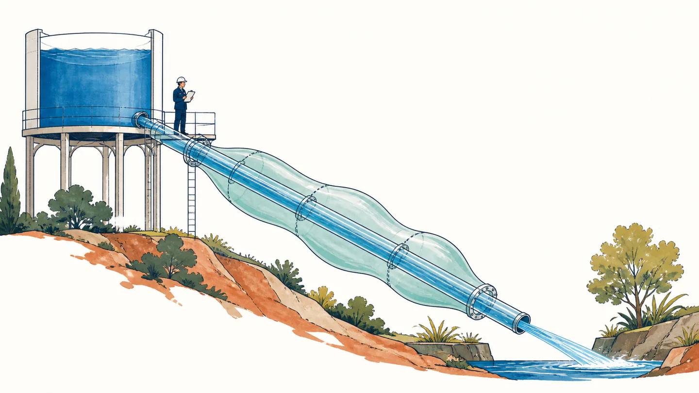
Pitot tubes: turning pressure difference into speed
A Pitot tube brings moving fluid to a stagnation point. At that point the local speed is approximately zero, so the ideal Bernoulli difference between the upstream static port and the stagnation port is
p0 − ps = ½ρV²V = √[2(p0−ps)/ρ]ps is static pressure; p0 is stagnation pressure. Neither word “stagnation” nor “total” means absolute pressure.
Worked example 2: an airspeed check
Suppose a Pitot system measures Δp=540 Pa in air with ρ=1.20 kg/m³. If the static absolute pressure is ps,abs=94.0 kPa, then
V=√(2×540/1.20)=√900=30.0 m/s½ρV²=½(1.20)(30.0)²=540 Pap0,abs=94.0 kPa+0.540 kPa=94.540 kPaPa/(kg/m³)=m²/s²; √ = m/sAt high Mach number, the air is no longer adequately modeled as incompressible, and a compressible-flow relation is required. Low differential pressure also makes sensor offset important; yaw, blockage, icing, and calibration alter the result. NASA’s Bernoulli notes introduce the equation, its streamline assumptions, and total pressure, while NASA’s Pitot-static guide documents low-speed limits and installation corrections. MIT’s hydrodynamics notes derive the pressure–speed relation and its assumptions.
Add pumps, turbines, and losses when the pipe is real
Real systems have friction, bends, valves, pumps, and turbines. The engineering head equation is better written as
p1/(ρg) + α1v1²/(2g) + z1 + hpump = p2/(ρg) + α2v2²/(2g) + z2 + hturbine + hLhL is head loss, hpump is added head, hturbine is extracted head, and α corrects for a nonuniform velocity profile.
The ideal equation is recovered when the added and removed heads, losses, and profile corrections are negligible. A pump can raise the total mechanical head; friction converts organized mechanical energy into internal energy. Pressure can therefore rise and speed can fall across a component without violating energy conservation, as long as the added or lost head is included.
For a nonuniform velocity profile, α is a kinetic-energy correction factor. A uniform one-dimensional profile has α=1; fully developed laminar pipe flow can approach α=2. Many turbulent pipe profiles are close to one, but a calculator should not silently assume that a centerline velocity is the section average. If a sensor reports a local speed near a wall or in a wake, the one-dimensional head equation needs a profile model or calibration.
The same bookkeeping explains why a pump is not a violation of Bernoulli. The pump adds shaft work to the fluid, while a turbine removes it. A valve, bend, screen, or sudden expansion creates irreversible loss head. If the selected points straddle one of these devices, the elementary constant form is missing a term; the extended equation is the correct repair.
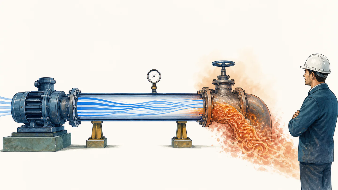
Assumptions and failure boundaries
hL and often calibration.The phrase “high speed means low pressure” is therefore conditional. It is reliable for a level, steady, low-loss comparison on the same streamline with no added work. An airplane wing, an eddying pipe bend, and a pump outlet may require a fuller control-volume analysis instead.
Common mistakes to catch before pressing calculate
| Failure | Why it fails | Repair |
|---|---|---|
| Mix gauge and absolute pressure | The two points do not share the same reference. | Use one pressure basis consistently; differences cancel only when the reference is shared. |
| Call stagnation pressure “absolute” | Stagnation describes velocity state, not pressure reference. | Write p0,g or p0,abs explicitly. |
| Use diameter ratio directly | Flow rate follows area, and circular area scales as diameter squared. | Use A=πD²/4. |
| Compare different streamlines | The Bernoulli constant may differ in rotational flow. | State the streamline or establish irrotational flow. |
| Ignore elevation | Pressure and speed changes can pay for a height change. | Keep the ρgz term until the geometry proves it cancels. |
| Forget losses or a pump | Real hardware changes total head. | Use the extended head equation and measured coefficients. |
| Assume incompressible air everywhere | Density changes become important with speed and pressure ratio. | Check Mach number and use compressible relations when needed. |
| Read a gauge face as data | Sensor offset, yaw, blockage, and icing bias Pitot measurements. | Calibrate and validate the installation. |
Bernoulli’s equation is a compact energy audit. Start by naming the fluid, streamline, pressure reference, elevations, and machines. Then use continuity to supply speeds, keep every term in compatible units, and add losses whenever the real pipe gives energy somewhere else to go.
Sources and further reading
- OpenStax, “Bernoulli’s Equation,” University Physics Volume 1
- OpenStax, “Fluid Dynamics,” University Physics Volume 1
- OpenStax, “Measuring Pressure,” University Physics Volume 1
- NASA Glenn Research Center, Bernoulli’s Equation
- NASA Glenn Research Center, Pitot–Static Tube–Speedometer
- MIT OpenCourseWare, Hydrodynamics Reading 3
- Penn State, Energy Equation for Control Volumes
- NIST Technical Note 831, Differential-Pressure Flow Devices
- BIPM, The International System of Units