Coulomb's Law: How Charge and Distance Set Electric Force

Two charged objects can attract or repel across empty space. Double one charge and the force doubles; double the separation and the force falls to one quarter. Coulomb’s law turns those observations into a vector equation, but the calculator must still know the medium, the sign of each charge, and the direction between them.

Force on charge 2 from charge 1F⃗₁₂ = k_e q₁q₂ r⃗₁₂ / |r⃗₁₂|³

Here r⃗₁₂ = r⃗₂ − r⃗₁ points from charge 1 to charge 2.

The scalar magnitude is easier to recognize:

F = k_e|q₁q₂|/r²

same signsrepulsion

opposite signsattraction

The absolute value belongs in the magnitude. The product q₁q₂ keeps its sign in the vector form, where direction is carried by r̂.

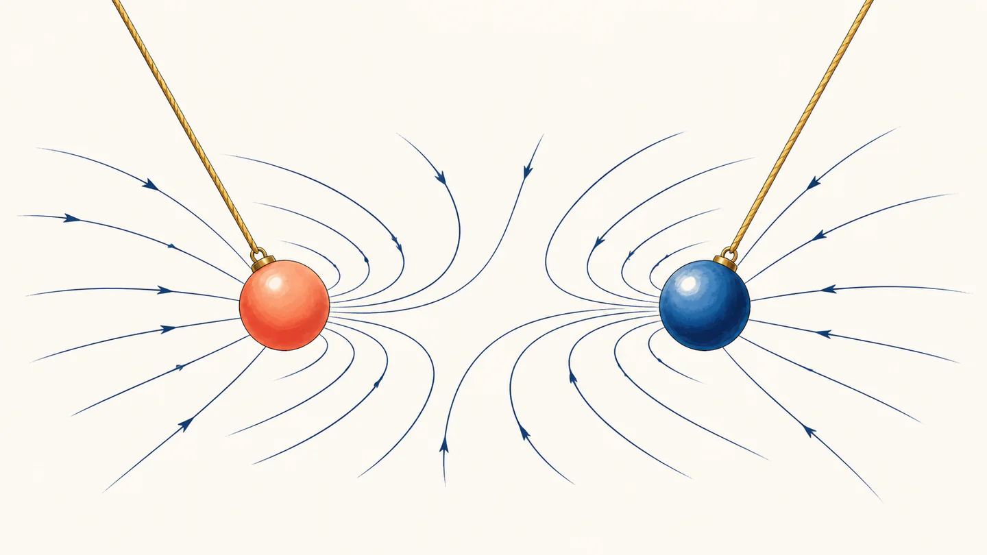
Two suspended colored charge spheres sit in a field of curved electric-field lines that bow around their interaction — The inverse-square magnitude is only half the story. The vector direction comes from the line joining the two charges and from whether their signs match.

Variables, units, and the reference direction

q₁, q₂point chargescoulombs, C

rseparation magnitudemetres, m

r⃗₁₂displacement from 1 to 2metres, m

F⃗₁₂force on 2 due to 1newtons, N

k_eelectrostatic constant in vacuumN·m²/C²

In vacuum, k_e=1/(4π ε₀)≈8.9875517923×10⁹ N·m²/C². The modern SI defines the ampere and elementary charge exactly, while ε₀ and the derived k_e have measured CODATA values. NIST’s CODATA constants and the BIPM SI Brochure are the appropriate references for current numerical constants.

Use coulombs in the equation. A microcoulomb is 1 μC=10⁻⁶ C; a nanocoulomb is 10⁻⁹ C. Convert centimetres to metres before squaring the separation. Because force scales as 1/r², a hidden factor of 100 in distance becomes a factor of 10,000 in force.

Choose a coordinate system before resolving components. If charge 1 is at r⃗₁ and charge 2 at r⃗₂, then

r⃗₁₂=r⃗₂−r⃗₁r=|r⃗₁₂|r̂₁₂=r⃗₁₂/r

The unit vector points from the source charge to the charge feeling the force.

The force on 1 due to 2 is equal and opposite: F⃗₂₁=−F⃗₁₂. That is Newton’s third law, not a second independent interaction.

Why the inverse square appears

An isolated point charge creates a spherical electric influence. The same amount of field flux spreads over a sphere whose area is 4πr², so field strength falls as 1/r². Multiplying the source charge and the test charge sets the interaction scale; the direction is radial.

The vector law can be written with the unit direction:

vector displacementr⃗₁₂

normalize directionr⃗₁₂/r³ = r̂₁₂/r²

insert charge productF⃗₁₂=k_eq₁q₂r̂₁₂/r²

read the signq₁q_2>0 → +r̂; q₁q_2<0 → −r̂

This is an electrostatic law: the charge locations and values are treated as stationary in the chosen frame. Accelerating charges radiate, and rapidly changing electromagnetic fields require Maxwell’s equations rather than an instantaneous inverse-square shortcut.

The potential-energy route gives a second derivation check. Bring q₂ from infinity to a distance r from q₁. Integrating the radial force gives

radial forceF(r)=k_e|q₁q₂|/r²

pair potential energyU(r)=k_eq₁q₂/r

force from potentialF⃗=−∇U

direction checksame signs repel; opposite signs attract

This route explains why electrostatic work is conservative: the energy change between two positions depends only on the endpoints. Once charges move rapidly enough for radiation or induction to matter, the instantaneous scalar-potential shortcut is no longer sufficient by itself.

Medium, permittivity, and screening

In a homogeneous, linear, isotropic material, replace the vacuum constant with

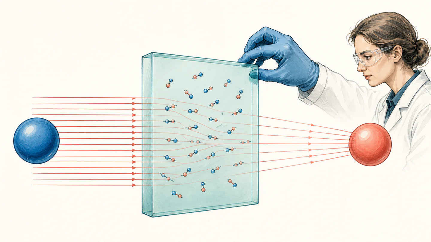
F = |q₁q₂|/(4π ε r²)ε=ε₀ε_r

ε_r is relative permittivity. Larger ε_r reduces the force by that factor in this idealized bulk model.

Do not divide by a material’s “dielectric constant” unless the intended approximation is clear. At high frequency, in anisotropic media, near interfaces, or in electrolytes with mobile ions, permittivity can depend on frequency, direction, position, and scale. Conductors rearrange free charge so that the electrostatic field inside their bulk is zero; grounded enclosures can shield a region without being described by a single scalar ε_r.

For an electrolyte, mobile ions can gather around a charge and screen the field over a Debye length. The interaction may then be closer to a screened inverse-square law, with an exponential attenuation factor, than to bare vacuum Coulomb behavior. In a polar liquid, a tabulated bulk relative permittivity is a useful first model but does not replace boundary conditions at an interface. A charge near a conductor interacts with induced surface charge; replacing the conductor by a point charge at its center is generally unjustified.

Electric field, potential, and energy are the same interaction viewed differently

The electric field is force per unit positive test charge:

field from one sourceE⃗=k_eq r̂/r²

Units: N/C or V/m.

potential from one sourceV=k_eq/r

Units: volts, J/C.

pair potential energyU=k_eq₁q₂/r

Units: joules, J.

The field is a vector; electric potential is a scalar. For a positive test charge, F⃗=qE⃗. The work done by the electrostatic force between two positions is W_field=−ΔU. A negative pair energy means opposite charges are bound relative to the chosen zero at infinite separation; it does not mean that energy has a negative unit.

The field viewpoint is especially useful when the test charge is changed. First solve the source-only field at the location, then multiply by the new test charge. A negative test charge reverses the force direction without changing the source field. This is why electric-field maps can be reused for many particles, while a force calculation always names the charge that feels it.

For a continuous line, sheet, or volume charge, the infinitesimal contribution is

dE⃗=k_e(dq/r²)r̂E⃗=∫dE⃗

The geometry, charge density, and integration limits determine how the inverse-square contributions cancel or reinforce.

A long uniformly charged wire, a finite disk, and a conducting shell therefore require different integrals or boundary-value methods. Substituting the total charge at the geometric center is only justified when symmetry or distance makes the object behave like a point to the required accuracy.

Superposition: add vectors, not magnitudes

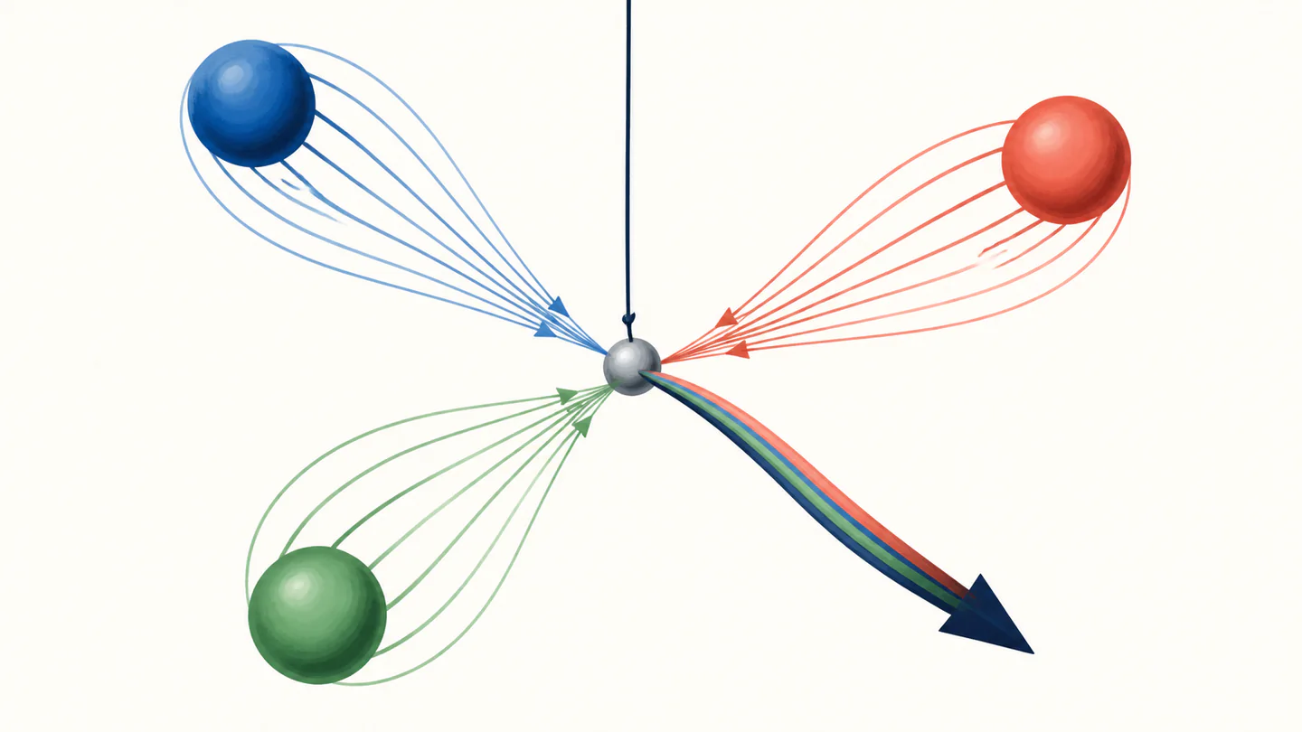
The force from many stationary point charges is the vector sum of each pairwise contribution:

F⃗_net=Σ_iF⃗_i→testE⃗_net=Σ_ik_eq_ir̂_i/r_i²

Resolve each term in the same coordinate basis before adding.

For symmetric arrangements, components can cancel while the vector magnitudes do not. A calculator that adds absolute forces first can be wrong by an entire direction. If charge is distributed continuously, replace the sum with an integral such as dE⃗=k_edq r̂/r²; the point-charge formula is then the kernel, not the final answer.

Three colored charge spheres send separate field ribbons to a suspended test bead that deflects along their vector sum — Superposition keeps each source contribution separate until the last step. The resultant force is a vector sum, not a sum of positive magnitudes.

Worked example 1: one attractive pair

Two point charges in vacuum are q₁=+2.00 μC and q₂=−3.00 μC, separated by r=0.500 m. Find the force magnitude and direction.

1 · convert chargesq₁=2.00×10⁻⁶ C; q₂=−3.00×10⁻⁶ C

2 · magnitudeF=(8.9875517923×10⁹)(|2.00×10⁻⁶·−3.00×10⁻⁶|)/(0.500)²

3 · evaluateF=0.215701243 N ≈0.216 N

4 · sign and directionq₁q_2<0 → attraction, toward q₁

5 · unit check(N·m²/C²)(C²/m²)=N

6 · distance checkr→2r would change F to F/4=0.0539253 N

The magnitude is positive by definition; the direction is supplied by the opposite signs. Reporting “−0.216 N” without saying which axis is negative would be incomplete.

Worked example 2: a vector sum on a line

Place q₁=+3.00 μC at x=0, q₂=−2.00 μC at x=0.400 m, and a positive test charge q_t=+1.00 μC at x=0.100 m. Find the net force on the test charge.

1 · source 1 distancer_1t=0.100 m; like signs repel → F₁ points +x

2 · source 1 magnitudeF₁=k(3.00×10⁻⁶)(1.00×10⁻⁶)/(0.100)²=2.69627 N

3 · source 2 distancer_2t=0.300 m; opposite signs attract → F₂ points +x

4 · source 2 magnitudeF₂=k(2.00×10⁻⁶)(1.00×10⁻⁶)/(0.300)²=0.199723 N

5 · vector sumF_net,x=+2.69627+0.199723=+2.89599 N

6 · back-substitutionF_net/F₁=1+0.199723/2.69627=1.07405

Both contributions point right in this arrangement, so the magnitudes happen to add. In a two-dimensional layout, resolve each vector into x and y components first; the same law does not permit adding lengths from different directions.

The same workflow works for electric field rather than force. First calculate each source field at the test location, then add the x and y components. Only after the vector sum is complete should you multiply by the signed test charge to obtain force. This separation lets one field solution serve test charges of different size and sign.

Rearrangements that expose what is measurable

Let F denote a measured magnitude in a known homogeneous medium. Useful inverse forms include

separationr=√[k_e|q₁q₂|/F]

charge magnitude|q₂|=Fr²/(k_e|q₁|)

relative permittivityε_r=k_vacuum|q₁q₂|/(Fr²)

field from a test forceE=F/|q_test|

These forms need domain checks: r>0, nonzero source charge, positive magnitude F, and a stated medium. A single force magnitude cannot reveal the sign of a charge or distinguish several unknown charges without additional direction or field measurements.

A scientist slides a translucent dielectric slab between two charges while field lines soften and spread through the material — A dielectric polarizes in response to the field. In a homogeneous ideal medium, that response appears as the relative-permittivity factor.

Common errors and physical limits

Failure	Why it fails	Repair
Use centimetres or microcoulombs as if they were SI base units	The powers of ten enter both charge product and distance squared.	Convert C and m before evaluating.
Report a magnitude as a signed scalar	A negative number without an axis or direction is ambiguous.	Report magnitude plus attraction/repulsion or a vector component.
Add force magnitudes from many charges	Opposing components may cancel.	Resolve and sum vectors in one basis.
Use the vacuum constant inside a material	Polarization changes the effective interaction.	Use `ε=ε₀ε_r` only when the medium model supports it.
Apply point-charge law to a nearby extended conductor	Charge redistributes over the surface and boundary conditions matter.	Use a field solution, image method, or measured calibration.
Ignore screening in an electrolyte	Mobile ions can attenuate the field over a characteristic length.	Use an electrochemical screening model.
Use electrostatics for rapidly changing currents	Radiation and magnetic induction are omitted.	Use Maxwell's equations or an appropriate quasistatic approximation.
Allow `r=0`	The ideal point model is singular and real charge has finite structure.	Reject coincident points and model finite-size physics.

The law is exact for ideal stationary point charges in the stated electrostatic model. It is an excellent local approximation for separated, small charged bodies, but it is not a complete theory of conductors, continuous charge distributions, radiation, or material interfaces. State the approximation before trusting the decimal places.

At very small separations, the point-charge idealization can fail because a real body has finite size, charge density, quantum structure, or a contact constraint. At very large separations in a material, boundaries and screening can dominate before the vacuum formula becomes the limiting description. At speeds where retardation is appreciable, the force is not transmitted instantaneously; use the full time-dependent electromagnetic fields. These are model-selection boundaries, not calculator rounding problems.

The sign convention should be visible in an interface as well as in prose. A robust calculator can report the positive magnitude, a direction such as “toward charge 1” or “+x,” and the medium used for ε. It should reject a zero separation, preserve the sign of each component, and keep guard digits until the final display. Those checks protect the physical interpretation without pretending that a decimal output proves the point-charge model applies.

The last displayed digit is therefore a report, not a new physical law. Match rounding to the uncertainty in the charges, distance, and material model.

That is the difference between a valid calculation and a misleadingly precise one.

Units, signs, geometry, and assumptions must agree.

Always.