How Error Propagates Through a Formula

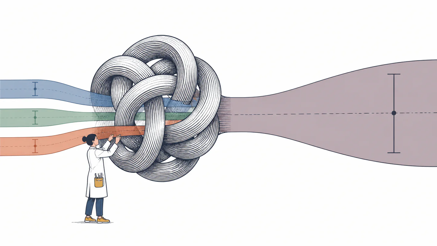
A formula can turn careful measurements into a result that looks far more certain than its inputs deserve. Measure a rectangle, multiply its sides, and the area acquires uncertainty from both measurements. Subtract two temperatures taken with the same instrument and some shared drift may cancel. Divide by a quantity near zero and a modest input uncertainty can produce a wild output distribution.

The familiar phrase error propagation hides an important distinction. A measurement error is the generally unknown difference between a measured value and the quantity’s reference value. What we can evaluate and propagate is measurement uncertainty: a model of the dispersion of values reasonably attributable to each input. NIST explicitly warns against confusing the two, while the international GUM calls the calculation the law of propagation of uncertainty.

Start with a measurement model, not a shortcut

Write the output as a function of its inputs:

The derivative ci asks a local question: if input xi moves slightly while the others stay fixed, how quickly does the output move? A first-order Taylor expansion makes the mechanism visible:

This is the general first-order covariance formula in NIST Technical Note 1297, Appendix A and JCGM 100. In matrix notation it is uc²(y) = cTUxc, where Ux is the input covariance matrix.

Units expose whether the calculation makes sense

Every term inside the variance formula has the square of the output unit; taking the square root returns uc(y) in the same unit as y. If the terms cannot be reduced to one common squared unit, the model or a conversion is wrong.

An uncertainty budget should therefore show more than one final ± number. It should list the input estimates, the meaning of their uncertainties, units, signed sensitivities, dependence assumptions, and contributions in the output unit.

The familiar rules are special cases

If inputs are independent, all covariance terms vanish and the combined standard uncertainty becomes a root-sum-of-squares calculation:

The product rule covers multiplication, division, and powers: an exponent p multiplies the first-order relative uncertainty by |p|. It requires nonzero input and output estimates. Near zero, percentages explode or lose meaning; return to the absolute sensitivity formula or propagate distributions directly.

Independence is an assumption, not the default state of the universe. Repeated readings may share calibration, reference data, environmental correction, sample preparation, or a fitted parameter. Independence implies zero covariance, but observing zero covariance does not generally prove independence.

Worked example 1: area from two independent lengths

Suppose the stated ± values are standard uncertainties, not tolerances:

The model is A = LW, so the best area estimate is A = (2.000)(1.200) = 2.400 m². Now calculate the sensitivities and contributions rather than multiplying the ± values blindly:

The relative check gives the same result: √[(0.005/2.000)² + (0.003/1.200)²] = 0.0035355, or 0.3536%; multiplying by 2.400 m² returns 0.008485 m². The two equal contributions also provide a useful audit: neither measurement dominates this budget.

Correlation can enlarge a sum and shrink a difference

Write covariance as u(x1,x2) = r12u1u2. For two readings:

Positive correlation increases uncertainty in a sum but can cancel shared motion in a difference. JCGM 100 specifically identifies shared instruments, standards, and reference data as possible sources of correlation. Omitting a material covariance term is not conservative in any reliable sense: depending on the model, it may understate or overstate the result.

Worked example 2: a correlated temperature difference

Two readings from a shared measurement system are T1 = 80.0 °C and T2 = 72.0 °C. Each has standard uncertainty 0.20 °C, and their estimated correlation coefficient is r = 0.75. For a temperature difference, an interval of 1 °C has the same magnitude as 1 K.

The correlated result is half the independence result because a shared component cancels in subtraction. This does not make either individual temperature twice as accurate. At the limiting checks, equal uncertainties with r = +1 cancel completely in the difference, while r = −1 produce 0.40 °C.

A ± sign does not tell you what kind of uncertainty you have

NIST commonly reports expanded uncertainty using k = 2, but TN 1297 says the resulting interval is only approximately 95% under suitable distribution and degrees-of-freedom conditions. It is not an exact universal promise.

If the area example’s ± values were hard tolerances instead of standard uncertainties, a first-order worst-case calculation would add absolute contributions: 0.006 + 0.006 = 0.012 m². Exact corner evaluation gives Amin = (1.995)(1.197) = 2.388015 m² and Amax = (2.005)(1.203) = 2.412015 m². That asymmetric bounded interval answers a different question from the 0.0085 m² combined standard uncertainty. JCGM 106 likewise treats tolerance and measurement uncertainty as separate inputs to conformity assessment.

When first-order propagation stops being trustworthy

The derivative formula is a local linear approximation. It earns trust when the model is smooth and nearly linear over the region containing meaningful input probability. It can mislead when:

The JCGM 101 Monte Carlo supplement provides an alternative: assign defensible input probability distributions and their dependence, sample them, run every draw through the full measurement model, and summarize the output distribution. It avoids derivatives and can produce asymmetric coverage intervals. It does not repair an omitted input, an unjustified distribution, a wrong correlation model, insufficient sampling, or a physically incomplete equation.

A disciplined propagation workflow

The calculation is not finished when a square root appears. It is finished when the reader can see which uncertainty was propagated, how each input affected the output, which dependencies were retained, and where the approximation might fail.