Measurements rarely arrive at the exact time, voltage, depth, or concentration someone wants. Linear interpolation fills that gap with a deliberately modest claim: between two known points, treat the relationship as a straight segment. It is an estimate between anchors—not permission to invent a trend beyond them.
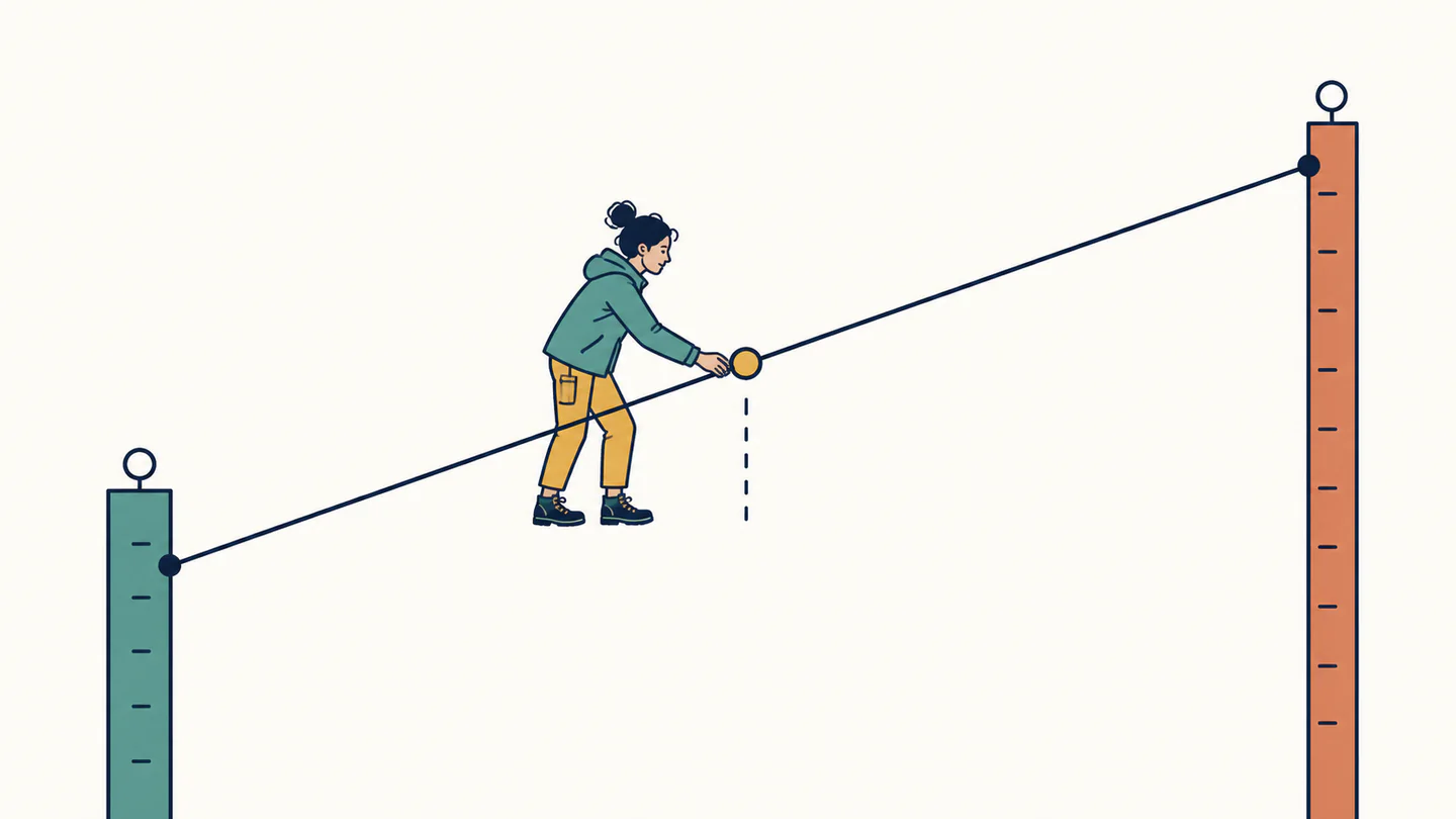
(x₀,y₀) and (x₁,y₁), with x₁ ≠ x₀y(x) = y₀ + (x − x₀)(y₁ − y₀)/(x₁ − x₀)The result is defined as interpolation only when the target x lies between the two x-values.
A fraction of the distance becomes a fraction of the change
The cleanest form introduces a dimensionless position:
t = (x − x₀)/(x₁ − x₀)y = (1 − t)y₀ + ty₁0 ≤ t ≤ 1t < 0 or t > 1 = extrapolationIndependent-variable coordinates in one common unit: hours, volts, metres, or another compatible unit.
Measured values in one common output unit: °C, kPa, dollars, and so on.
Fractional position with no unit. The weights 1 − t and t add to one.
The dimensional check catches mixed-unit errors. The slope (y₁ − y₀)/(x₁ − x₀) has units of y per x. Multiplying by x − x₀ restores y units, so it can be added to y₀. At x = x₀, the answer must be y₀; at x = x₁, it must be y₁.
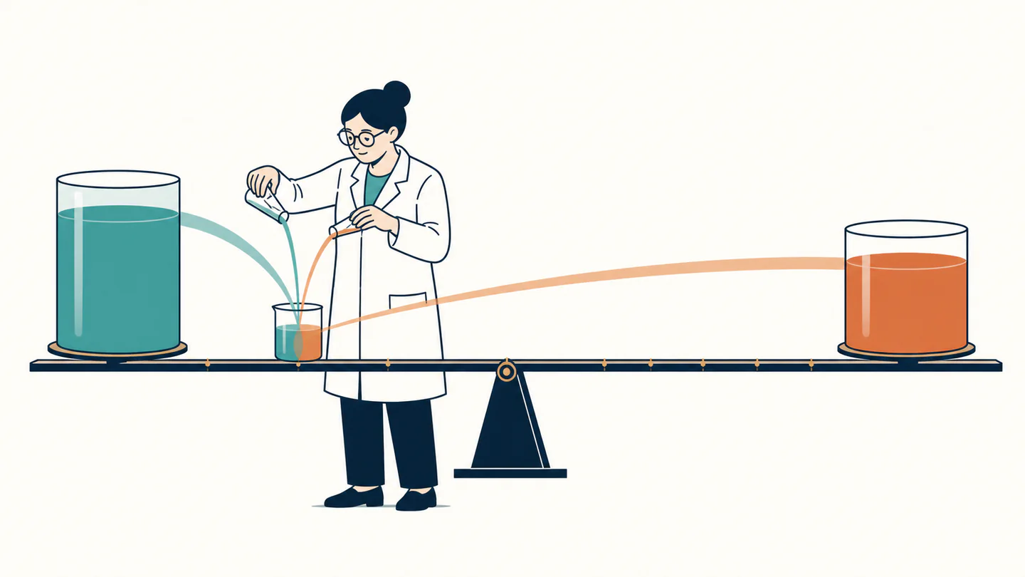
Worked example 1: a temperature between observations
At 09:00 the recorded temperature is 20 °C; at 13:00 it is 40 °C. Estimate 10:30, explicitly assuming linear change over this four-hour window.
t = (10.5 − 9)/(13 − 9) = 1.5/4 = 0.375y = 20 + 0.375(40 − 20) = 27.5 °C0.625(20) + 0.375(40) = 27.5 °C20 < 27.5 < 40The answer is a straight-line estimate, not evidence that the temperature rose steadily every minute. A passing cloud, a heater cycle, or an unobserved front can make the actual curve bend.
Worked example 2: a local calibration lookup
Two calibration points say 1.0 V corresponds to 0 kPa and 5.0 V corresponds to 200 kPa. For 3.2 V:
t = (3.2 − 1.0)/(5.0 − 1.0) = 2.2/4.0 = 0.55p = 0 + 0.55(200 − 0) = 110 kPa200 kPa / 4.0 V = 50 kPa/V0 + 2.2 V × 50 kPa/V = 110 kPaNIST describes calibration as a relationship between known input and instrument response; a linear approximation is valid only over a supported range. See NIST’s calibration overview and linearity guidance.
What the straight line assumes
The target lies between measured x-values. NIST’s [interpolation reference](https://www.itl.nist.gov/div898/software/dataplot/refman2/auxillar/interpol.htm) distinguishes this from extrapolation.
Equal input steps should produce approximately equal output steps in the chosen interval.
A switch state, phase boundary, eligibility rule, or jump discontinuity cannot be made meaningful by drawing a line through it.
Endpoint error, rounding, and calibration uncertainty carry into the interpolated result.

Common errors
| Error | Repair |
|---|---|
| Use two readings with the same x-value | The denominator is zero; investigate repeated-measurement variation instead. |
| Mix minutes and hours, or mV and V | Convert x-values to one unit before subtracting. |
| Call an outside value interpolation | Name it extrapolation and justify a model beyond the data. |
| Assume two points prove linearity | They always determine a line; use physics or more data to support it. |
| Report extra decimal places | Round to the evidence and propagate stated measurement uncertainty. |
Linear interpolation is deliberately local. It is excellent for a transparent estimate inside a defended interval; it should be replaced by a measured curve, a piecewise model, or a physical model when curvature, thresholds, saturation, or discontinuities matter. USGS likewise notes that interpolation rules depend on domain coverage and continuous behavior in its methods reference.