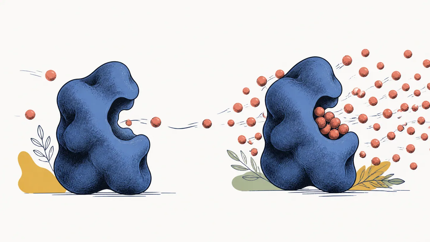
The Michaelis–Menten Equation: How Enzyme Rate Saturates

An enzyme can make a reaction much faster without being consumed. Add substrate to a fixed amount of enzyme and the initial rate usually rises quickly, then levels off: every active site is busy often enough that extra substrate has nowhere useful to go. The Michaelis–Menten equation is a compact model of that saturation curve. It is also a good example of what a calculator must keep visible: a mechanism, a choice of units, a limiting value, and a validity boundary.

Initial-rate modelv₀ = V_max[S]₀ / (K_M + [S]₀)

The concentration ratio is the fraction of the limiting rate reached at the chosen substrate concentration.

A sculptural enzyme has a sparse substrate stream on one side and crowded occupied active sites on the other — At low substrate concentration, more substrate usually means a faster initial rate. At high concentration, occupied active sites make the curve flatten.

The mechanism behind the equation

The minimal one-substrate scheme is

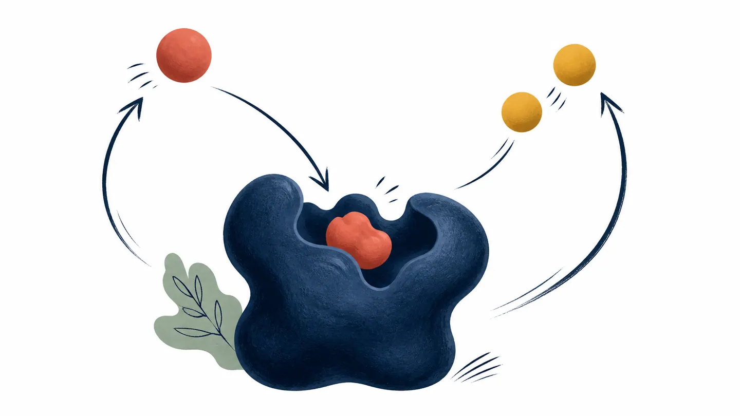
E + S ⇌ ES → E + P

E is free enzyme, S is substrate, ES is the enzyme–substrate complex, and P is product.

The forward binding step has rate constant k₁, the complex can dissociate with k₋₁, and productive turnover has catalytic constant k_cat. Under the Briggs–Haldane steady-state approximation, the complex parameter is

K_M = (k₋₁ + k_cat) / k₁V_max = k_cat[E]_T

Here [E]_T = [E] + [ES] is total active enzyme. Because k₋₁ and k_cat have units of s⁻¹ while k₁ has units of M⁻¹ s⁻¹, K_M has concentration units. Only in the rapid-equilibrium special case where dissociation dominates turnover does K_M reduce to the binding dissociation constant. A low K_M can suggest stronger apparent affinity, but it is not automatically a molecular binding constant.

Deriving the steady-state rate law

Mass action gives the complex balance

1 · formation and lossd[ES]/dt = k₁[E][S] − (k₋₁ + k_cat)[ES]

2 · steady state0 ≈ k₁[E][S] − (k₋₁ + k_cat)[ES]

3 · substitute K_M[E][S] = K_M[ES]

4 · conserve enzyme([E]_T − [ES])[S] = K_M[ES]

5 · solve complex[ES] = [E]_T[S] / (K_M + [S])

6 · form productv₀ = k_cat[ES] = V_max[S] / (K_M + [S])

The approximation is not a claim that [ES] never changes. It says that after a short formation transient, complex formation and loss nearly balance while substrate remains close to its starting value. The measured quantity is therefore an initial rate v₀, not the slope after most substrate has been consumed.

Symbols, units, and a dimension check

v₀initial rateμM s⁻¹ or M s⁻¹

V_maxlimiting initial ratesame rate unit as v₀

[S]₀initial substrateμM, mM, or M

K_Mhalf-rate concentrationsame concentration unit as [S]₀

k_catturnover numbers⁻¹

The ratio [S]₀/(K_M + [S]₀) is dimensionless. Therefore, if V_max is in μM s⁻¹, the result is in μM s⁻¹. Put K_M and [S]₀ in the same concentration unit before adding them; converting one to M and leaving the other in μM creates a thousand-fold error even though the formula looks correct.

What the curve says at three useful points

At the half-rate point, set [S]₀ = K_M:

[S]₀ ≪ K_Mv₀ ≈ (V_max/K_M)[S]₀first-order in substrate

[S]₀ = K_Mv₀ = V_max/2half the limiting rate

[S]₀ ≫ K_Mv₀ ≈ V_maxapproximately zero-order in substrate

The word “maximum” can mislead: in the ideal hyperbola, V_max is approached asymptotically. A finite experiment can get close, but it does not prove that an exactly maximum rate has been observed.

An enzyme binds a substrate bead, transforms it in the active pocket, and releases product beads around a circular motion — The enzyme is regenerated after product leaves. The initial-rate equation summarizes many such binding and turnover cycles.

Rearrangements for an interactive calculator

The same law can answer inverse questions. Let the saturation fraction be f = v₀/V_max. Then

ratev₀ = V_max[S]₀/(K_M + [S]₀)

substrate[S]₀ = K_Mv₀/(V_max − v₀)

Michaelis constantK_M = [S]₀(V_max − v₀)/v₀

limiting rateV_max = v₀(K_M + [S]₀)/[S]₀

fractional formf = [S]₀/(K_M + [S]₀)

fraction inverse[S]₀ = K_Mf/(1 − f)

The inverse for substrate requires 0 ≤ v₀ < V_max; a displayed rate at or above the limiting rate cannot produce a finite positive substrate concentration under this model. Estimating parameters from many measured rates should use nonlinear regression on the original hyperbola. Reciprocal plots such as Lineweaver–Burk are useful historical teaching transforms, but they magnify uncertainty at small rates and should not be treated as a safer fitting method by default.

Worked example 1: forward rate and inverse check

Suppose V_max = 2.40 μM s⁻¹, K_M = 15.0 μM, and [S]₀ = 45.0 μM.

1 · denominatorK_M + [S]₀ = 15.0 + 45.0 = 60.0 μM

2 · saturation fractionf = 45.0/60.0 = 0.750

3 · ratev₀ = 2.40 × 0.750 = 1.80 μM s⁻¹

4 · inverse check[S]₀ = 15.0 × 1.80/(2.40 − 1.80) = 45.0 μM

5 · interpretationv₀/V_max = 0.750, not 1.000

6 · unit check(μM s⁻¹) × (μM/μM) = μM s⁻¹

The result is 75% of the limiting rate. The remaining 25% is not a rounding mistake; it is the gap between a finite concentration and an asymptote.

Worked example 2: competitive inhibition

For an ideal competitive inhibitor that binds free enzyme, use

v_i = V_max[S]₀ / (K_M(1 + [I]/K_i) + [S]₀)K_M,app = K_M(1 + [I]/K_i)

The ideal model leaves V_max unchanged and shifts the half-rate concentration upward.

Take V_max = 1.80 μM s⁻¹, K_M = 12.0 μM, [S]₀ = 18.0 μM, [I] = 6.00 μM, and K_i = 3.00 μM.

1 · inhibitor factorα = 1 + 6.00/3.00 = 3.00

2 · apparent constantK_M,app = 12.0 × 3.00 = 36.0 μM

3 · inhibited ratev_i = 1.80 × 18.0/(36.0 + 18.0) = 0.600 μM s⁻¹

4 · no inhibitorv₀ = 1.80 × 18.0/(12.0 + 18.0) = 1.08 μM s⁻¹

5 · inverse checkK_M,app = 18.0(1.80 − 0.600)/0.600 = 36.0 μM

6 · interpretationV_max stays 1.80 μM s⁻¹ in the ideal competitive model

At this substrate concentration, inhibition lowers the rate from 1.08 to 0.600 μM s⁻¹. More substrate can overcome ideal competition in the limit, but a mixed, uncompetitive, allosteric, or substrate-inhibited mechanism changes a different set of parameters. “An inhibitor is present” is not enough information to choose this equation.

A coral inhibitor plug blocks an enzyme pocket while substrate beads wait nearby and a side path remains open — Competitive inhibition changes the apparent half-rate concentration in the ideal model. It does not automatically describe every inhibitor.

Relating V_max to enzyme amount

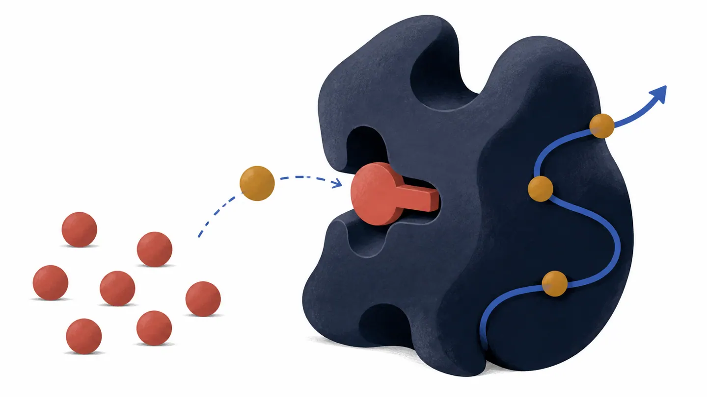
The relationship V_max = k_cat[E]_T gives the limiting rate a physical interpretation. If k_cat is in s⁻¹ and active enzyme concentration is in μM, their product is μM s⁻¹. Doubling active enzyme at fixed temperature and assay conditions doubles V_max but leaves K_M unchanged in the simple model. This is why kinetic experiments often run several enzyme concentrations: a proportional change in the limiting rate supports a catalytic-capacity interpretation, while a changing apparent K_M can signal assay interference, depletion, or a mechanism that is not being held constant.

Do not silently substitute total protein for active enzyme. A preparation can contain inactive, misfolded, or inhibited molecules. The fitted V_max reports the capacity of the active fraction under the assay conditions, not an absolute guarantee about every protein molecule in the tube. When comparing experiments, hold temperature, pH, ionic strength, cofactor concentration, and detector response fixed before interpreting a change in V_max as a change in enzyme amount or turnover.

Designing a substrate series

A useful substrate series spans below, near, and above K_M. Points only far below K_M mostly identify the ratio V_max/K_M; they cannot separate the two parameters well. Points only far above K_M cluster near the asymptote and reveal little about the half-rate location. Include replicate initial slopes, randomize or balance run order when drift is possible, and keep substrate depletion small in each slope window.

Before fitting, plot rate against substrate concentration with the units visible. Look for a plausible rectangular hyperbola, curvature caused by inhibition, or a baseline that changes with concentration even when enzyme is absent. A blank reaction can reveal optical or chemical background that would otherwise be mistaken for catalytic rate. Replicates help distinguish a real change in curve shape from pipetting noise; they do not make an unsuitable model valid.

The fitted parameters are conditional on the experiment. A K_M measured at one pH or temperature need not transfer to another, and changing the reporting unit changes the numerical value of a concentration parameter while leaving the physics unchanged. Always report the unit, buffer, temperature, enzyme amount, substrate range, and whether the number is a fit, a literature value, or a value calculated from a displayed rate.

A quick model-selection checklist

Use the base equation when the reaction has one dominant substrate, a measurable initial interval, negligible product, and no obvious cooperativity or inhibition. Use the competitive extension only when an inhibitor is known or supported to compete for free enzyme. If the curve is sigmoidal, test a cooperative model rather than forcing a rectangular hyperbola. If the rate falls at very high substrate, consider substrate inhibition or an assay artefact. If the signal is curved from the first seconds, consider a pre-steady-state or integrated progress model.

These choices are not cosmetic. A calculator can return a numerically precise K_M from a poor model, and an extra decimal place cannot repair a wrong mechanism. Treat a residual pattern, an unexpected fitted parameter, or a parameter that changes with enzyme concentration as evidence to investigate—not as a reason to keep pressing “calculate.”

Assumptions to state beside a result

The equation is most defensible when the assay is well mixed, temperature and pH are controlled, enzyme activity remains constant, and one substrate dominates the measured reaction. Use an initial interval with little substrate depletion—often operationally less than about 10%—so product accumulation, reverse reaction, and product inhibition are negligible. Substrate should be in excess of enzyme, the detector should respond linearly, and mass transfer should not be the rate-limiting step.

The steady-state condition requires a short transient after which [ES] changes slowly compared with its formation and loss. If enzyme and substrate concentrations are comparable, or if the transient itself is the quantity of interest, the reactant-stationary approximation can fail. A progress-curve slope taken after substantial depletion is not the same thing as v₀.

Common errors and guardrails

Error	Why it fails	Safer check
Mix μM and M	The denominator adds unlike concentration units.	Convert both `K_M` and `[S]₀` to one unit first.
Call K_M a universal binding constant	`k_cat` contributes to the Briggs–Haldane expression.	Call it a half-rate or fitted kinetic constant unless rapid equilibrium is shown.
Report V_max as a finite observation	It is the high-substrate asymptote.	Check that the measured rate is below the fitted limit.
Use a depleted-substrate slope as v₀	Substrate and product concentrations have changed.	Fit the early linear interval or an integrated progress-curve model.
Use competitive inhibition for every inhibitor	Binding to ES or an allosteric site changes the equation.	Identify the inhibition mechanism before selecting a model.
Assume low K_M always means tight binding	Turnover and dissociation both enter K_M.	Compare with an independently measured dissociation constant.
Fit reciprocal plots without checking uncertainty	Small rates receive disproportionate leverage after inversion.	Prefer nonlinear regression of the original hyperbola.

Limits and useful extensions

Allosteric or cooperative enzymes can have a sigmoidal response better described by a Hill-type model. Multi-substrate reactions, reversible product formation, substrate inhibition, enzyme deactivation, crowding, and diffusion limits require additional terms or a different model. Pre-steady-state experiments resolve the formation transient; integrated progress-curve models follow changing substrate and product; single-turnover experiments answer a different question altogether. A smooth-looking fit cannot decide among mechanisms by itself: it only says how well the chosen rate law summarizes the measured interval.