The Radioactive Decay Law: Predicting Nuclei, Activity, and Half-Life

Radioactive decay is random for one nucleus and remarkably regular for a large population. You cannot predict which atom will transform next, but you can predict the expected fraction of a parent nuclide that remains after a measured time. The single-parent decay law turns that distinction into a calculator: it connects the number of undecayed nuclei, the activity in becquerels, the decay constant, and the half-life.

Single-parent modelN(t) = N₀e^−λt · A(t) = λN(t)

Keep λ and t in reciprocal, matching time units; the exponent must be dimensionless.

Two glowing vessels show a large parent population and its smaller half-life remainder connected by a sweeping time arc — Half-life is a population statement: after one half-life, the expected parent population is half its starting value.

What the symbols mean

N(t)parent nuclei remaining at elapsed time tcount, dimensionless

N₀parent nuclei at the reference timesame count unit as N(t)

λdecay constants⁻¹, h⁻¹, y⁻¹, or another reciprocal time

A(t)intrinsic activityBq = s⁻¹

T_1/2half-lifetime

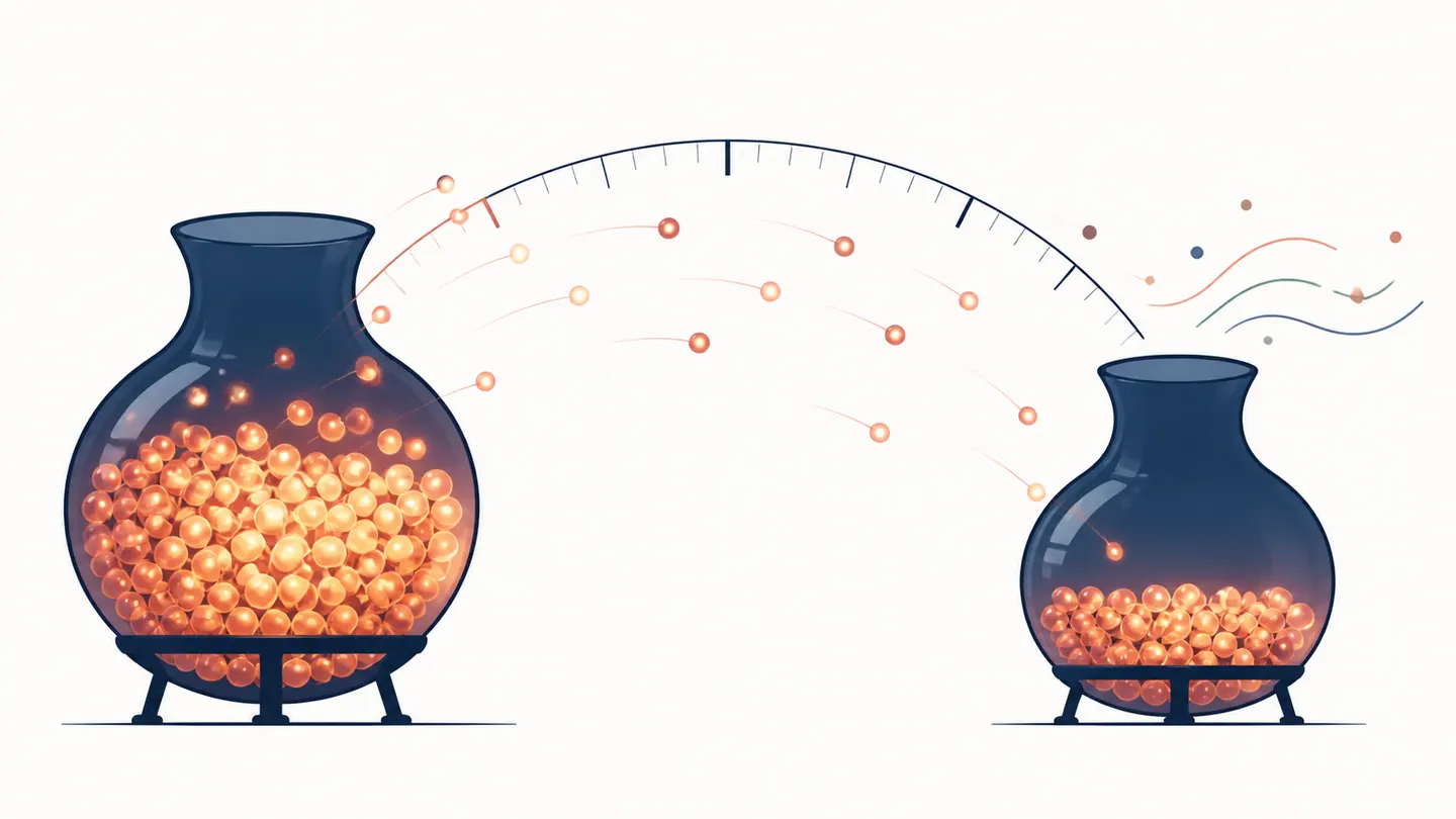
N(t) counts the parent nuclide only; it does not count daughter nuclei created by decay. λ is the conditional probability rate for a surviving nucleus in the constant-hazard model. The product λt has no unit. If the half-life is entered in hours, use hours for t and h⁻¹ for λ, or convert both to seconds before calculating activity in Bq.

Deriving the exponential law from constant hazard

Assume that, over a short interval dt, each surviving nucleus has decay probability λdt plus smaller-order terms. The expected population loss is proportional to the population still present:

1 · expected lossdN = −λN dt

2 · separate variablesdN/N = −λ dt

3 · integrateln(N/N₀) = −λt

4 · exponentiateN(t) = N₀e^−λt

5 · differentiate−dN/dt = λN(t)

6 · define activityA(t) = λN(t) = A₀e^−λt

The smooth curve is an expectation for a population. Individual transformations are independent random events, and a small detector sample can fluctuate around the curve. The exponential is not a claim that an identical fraction decays in every short interval or that a single atom has a predictable deadline.

Half-life, decay constant, and mean lifetime

Set N(T_1/2) = N₀/2 in the law:

T_1/2 = ln 2 / λλ = ln 2 / T_1/2τ = 1/λ = T_1/2/ln 2

The mean lifetime τ is about 1.4427T_1/2. After one mean lifetime, the remaining fraction is e⁻¹ ≈ 0.3679, not one-half. After n half-lives, both parent population and intrinsic activity have fallen by 2⁻ⁿ for a pure parent source.

Activity is not the same as a nucleus count

Activity is the expected transformation rate:

intrinsic activityA(t) = −dN/dt = λN(t)

initial activityA₀ = λN₀

SI reporting1 Bq = 1 s⁻¹

Use λ in s⁻¹ when reporting Bq. A curie is an older activity unit: 1 Ci = 3.7 × 10¹⁰ Bq. The named becquerel distinguishes activity from any other quantity with reciprocal-second dimensions. The activity of a pure parent source and its parent count have the same exponential fraction, but they are different quantities with different units and interpretations.

A glass chamber of glowing nuclei sends irregular individual sparks into a smooth navy population sweep observed by a scientist — Random individual decays aggregate into a smooth exponential expectation. A detector still adds efficiency, background, and counting uncertainty.

Rearrangements for a decay calculator

Define the dimensionless remaining fraction f = N/N₀. For a pure parent source with comparable activity calibration, f = A/A₀ as well:

remaining fractionf = e^−λt = 2^−t/T_1/2

elapsed timet = −ln(f)/λ = T_1/2ln(1/f)/ln2

initial countN₀ = N e^λt

initial activityA₀ = A e^λt

inferred λλ = ln(N₀/N)/t

inferred half-lifeT_1/2 = t ln2 / ln(N₀/N)

The domain for a finite elapsed time is 0 < f ≤ 1. Form the ratio before taking a logarithm: ln(0.300 MBq) is not meaningful, while ln(A/A₀) is dimensionless. An inferred half-life is meaningful only when the two measurements refer to the same parent population and the same activity definition.

Worked example 1: population and intrinsic activity

Given N₀ = 8.00 × 10¹² parent nuclei, T_1/2 = 6.00 h, and t = 15.0 h, find N(t) and A(t).

1 · convert half-lifeλ = ln2/6.00 h = 0.115524530 h⁻¹

2 · count half-livesn = 15.0/6.00 = 2.50

3 · remaining fractionf = 2⁻²·⁵⁰ = 0.176776695

4 · parent countN = (8.00 × 10¹²)f = 1.41421 × 10¹²

5 · convert λ for Bqλ = 0.115524530/3600 = 3.20901472 × 10⁻⁵ s⁻¹

6 · activityA = λN = 4.53823 × 10⁷ Bq = 45.3823 MBq

Checks: N/N₀ = 0.176776695 agrees with e^−λt. The initial activity is A₀ = λN₀ = 2.56721 × 10⁸ Bq, and A/A₀ = 45.3823/256.721 = 0.1767767. The activity is not the count of nuclei; it is the expected number of transformations per second.

Worked example 2: infer elapsed time from activity

Suppose a single parent source starts at A₀ = 2.40 MBq, has half-life 12.0 h, and later measures A = 0.300 MBq. Find the elapsed time.

1 · make a ratiof = A/A₀ = 0.300/2.40 = 0.125000 = 1/8

2 · convert half-lifeλ = ln2/12.0 h = 0.057762265 h⁻¹

3 · invert lawt = −ln(0.125000)/0.057762265 = 36.0 h

4 · half-life check0.125 = 2⁻³, so t = 3 × 12.0 h = 36.0 h

5 · forward checkA(36 h) = 2.40 × 2⁻³ = 0.300 MBq

6 · domain check0 < A/A₀ ≤ 1

This is an inverse model calculation, not a detector calibration. If “0.300 MBq” is really a raw count rate, first correct for efficiency, geometry, emission probability, dead time, and background.

Measuring activity in the real world

Intrinsic activity A = λN is an expected physical transformation rate. An instrument usually reports counts per second or an inferred activity. The conversion depends on detector efficiency, source-to-detector geometry, emission probability for the selected radiation line, background, dead time, coincidence effects, and calibration uncertainty. Sparse counts also fluctuate: for an ideal Poisson count, the variance equals the mean.

Always attach a reference time to an activity value. A detector reading can be correct for its timestamp and still be misused in a decay calculation if the timestamp is omitted. Use Bq for the calibrated activity, not a count rate that has not been corrected. Report uncertainty when the measurement, rather than the decay law, is the limiting source of precision.

Decay chains and branching are different models

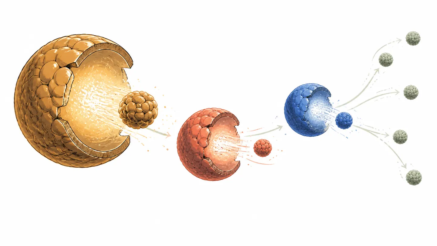
The one-parent law does not describe a mixture or a daughter chain automatically. A parent may have multiple decay branches; a daughter may itself be radioactive. In a chain, coupled balance equations (often called Bateman equations) determine daughter ingrowth and activity. At secular equilibrium, daughter and parent activities can become similar even though their decay constants differ. A graph that appears to have one smooth half-life can therefore be an effective summary of several nuclides, not a physical half-life of one parent.

For biological clearance, leakage, chemical separation, or another independent first-order removal process, an observed effective constant can sometimes be written λ_eff = λ_physical + λ_removal. Its effective half-life is not the nuclide’s physical half-life. State which constant the calculator is returning instead of hiding removal inside a generic “decay” field.

A glowing amber parent sphere transforms through coral and blue daughter stages into several possible descendants — A daughter chain needs coupled equations. A single exponential is safe only when the measured signal really belongs to one parent.

Reading a decay curve without over-interpreting it

A straight line appears only after taking the natural logarithm of a correctly normalized parent fraction: ln(N/N₀) = −λt. Its slope has reciprocal-time units and its intercept is zero only when the chosen reference really is t = 0 for the same population. If a graph uses detector counts, first correct for background and keep the efficiency and geometry constant; otherwise a change in the instrument can masquerade as a change in λ.

The ratio form is often more reliable than subtracting two large activity values. For example, if both measurements share a common calibration factor, that factor cancels in A/A₀. It does not cancel if the source moved, the emission line changed, the detector dead time changed, or a daughter contribution grew between measurements. An apparently tidy half-life can therefore be a property of the measurement setup rather than of the nuclide.

Use guard digits for λ and the fraction in an inverse calculation. When f is close to one, a small absolute error in two nearly equal activity readings can cause a large relative error in −ln f. When f is very small, background subtraction and finite counting statistics become dominant. A calculator should expose the ratio, timestamp, and uncertainty inputs instead of presenting an age as if it were exact.

Activity, dose, and count rate are not interchangeable

Activity describes transformations per unit time. Absorbed dose describes energy deposited per unit mass, and equivalent or effective dose includes radiation weighting and tissue factors. A high activity does not by itself determine a dose rate: particle energy, emission spectrum, shielding, distance, geometry, exposure time, and biological context also matter. This article’s A = λN relation is therefore not a dose calculator.

Likewise, a detector count rate is a measurement signal. To infer activity, a calibration model maps counts through efficiency, branching or emission probability, geometry, dead-time correction, and background. If any of those terms changes with time, the simple activity ratio is invalid. Keep the names visible in a user interface so that “Bq,” “counts per second,” and “dose” cannot be entered into one unlabeled field.

Common errors and guardrails

Error	Why it fails	Repair
Mix seconds and hours	The exponent gains an unintended factor of 3,600.	Use matching units for λ and t; use s⁻¹ for Bq.
Use T_1/2 where λ belongs	Half-life and decay constant are related but not equal.	Convert with λ = ln2/T_1/2.
Treat activity as a nucleus count	A has units of Bq; N is a count.	Use A = λN and state the unit.
Confuse τ with T_1/2	One mean lifetime leaves e⁻¹, not one-half.	Use τ = 1/λ = T_1/2/ln2.
Subtract a fixed number per interval	Decay removes a fraction of survivors, not a fixed count.	Use the exponential law or half-life powers.
Use detector counts as Bq	Efficiency, background, and geometry are missing.	Apply a stated calibration and uncertainty model.
Force a chain into one half-life	Daughter ingrowth and branches change the signal.	Use coupled chain equations or label an effective fit.
Round λ too early	Inverse logarithms magnify small parameter errors.	Keep guard digits until the final display.

Limits of the single-exponential model

The model assumes one identified parent, a constant decay constant, a fixed reference time, no external production or removal, and a large enough population that the expected curve is informative. It does not model detector response, daughter photons, self-absorption, changing chemistry, biological clearance, or a time-varying source. For a nuclide-specific half-life, use an evaluated nuclear-data record and report its reference and uncertainty; a generic calculator example is not a substitute for isotope identification.