Physics and mechanics
Electric Field Graph Calculator
Generate an exact plot-ready table of signed radial electric field and potential versus distance for one isolated point charge in a uniform dielectric, with a highlighted operating radius.
CURRENT MODEL
Enter the declared electric-field case
Electrostatics students, demonstration designers, and preliminary bench planners who need a transparent radial field profile rather than a decorative graph.
Decision supportedQuantify how rapidly the ideal point-charge field falls across a declared radius range and inspect the current point without evaluating the singular zero-radius boundary.
SUBJECT DECISION ILLUSTRATION
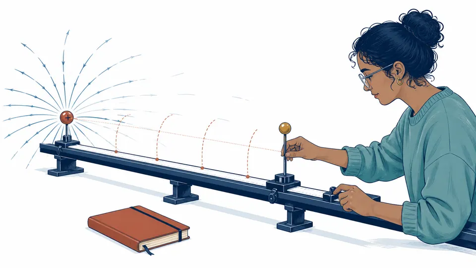
A radial field-mapping walk away from one source
This wave intentionally uses a static measurement scene instead of an interactive chart; the current numerical profile is preserved in the table.
| Radius (cm) | Radius (m) | Signed E_r (V/m) | |E| (V/m) | Potential (V) | Direction |
|---|
How to use
Build a defensible radial profile dataset
- Confirm that the source is adequately represented by one isolated point charge or by an external spherically symmetric equivalent.
- Enter the signed source charge from a documented estimate or measurement and identify the material represented by relative permittivity.
- Choose positive minimum and maximum radii that stay outside the physical source and bracket the region of interest.
- Set the current radius inside that range to obtain an exact operating-point field and potential.
- Read the endpoint ratio to understand distance sensitivity, then use the ledger rather than rounded card values for plotting.
- Label any external graph with units, axis scaling, dielectric assumption, source geometry, and the excluded zero-radius singularity.
Profile fundamentals
Five features of an isolated point-charge field
- Radial symmetry
- The ideal field depends only on distance from the point and points along the radial line.
- Inverse-square field
- Field magnitude falls as 1/r squared, making the near-source rows especially sensitive to distance error.
- Inverse-distance potential
- Potential falls as 1/r and remains a scalar, so it changes more slowly with radius than field magnitude.
- Signed direction
- Positive source charge produces outward E_r; negative charge produces inward E_r under the declared radial convention.
- Zero-radius singularity
- The mathematical point model is undefined at its source and must not be regularized with an arbitrary tiny radius.
Calculation method
Use one SI bridge for every profile row
Nanocoulombs are converted to coulombs and centimetres to metres before applying the Coulomb constant. Every sampled radius uses the same charge and dielectric assumption, producing signed radial field, magnitude, and potential in one auditable row.
The table is the page's plot-ready output. This wave deliberately avoids an interactive chart, so no clipped curve or axis choice can hide the exact values; users can export the ledger into the plotting environment appropriate to their analysis.
Distance uncertainty near the source
Because E scales with 1/r squared, a small radius error has roughly twice the relative influence on field as on potential. Mechanical reference points matter most in the first rows.
When a sphere behaves like a point
Outside a spherically symmetric charge distribution, the external field matches a point charge at the centre. Inside the body or for irregular electrodes, that shortcut no longer follows.
Linear dielectric assumption
Dividing by a single relative permittivity assumes a homogeneous, isotropic, linear medium. Interfaces can bend field lines and redistribute bound or free charge.
Detailed calculation process
Symbols, current substitution, intermediate quantities, and reconciliation
E_r(r)=k_e q/(epsilon_r r^2); V(r)=k_e q/(epsilon_r r)The profile uses SI metres and coulombs at full precision; values are rounded only when written to cards and rows.
| Symbol | Meaning | Default | Unit |
|---|---|---|---|
| q | Signed source charge | 2 nC = 2e-9 C | C |
| epsilon_r | Relative permittivity | 1 | dimensionless |
| r | Distance from source centre | 10 cm = 0.10 m | m |
| k_e | Coulomb constant used by the model | 8.9875517923e9 | N m2/C2 |
| E_r | Signed radial electric field | calculated | V/m |
| V | Potential relative to infinity | calculated | V |
Waiting for valid inputs.
Result interpretation
Use the field ratio to judge spatial sensitivity
A large near-to-far ratio is expected over a wide radius range and does not imply changing source charge. A negative signed field means inward direction, not negative magnitude. At zero source charge the whole ledger becomes zero and radial direction is deliberately left undefined.
Evidence to retain
Document geometry before exporting the profile
Keep the charge estimate and uncertainty, source radius and shape, centre reference, dielectric identity and frequency, temperature, humidity, conductor and boundary locations, radius measurement method, chosen range, sample count, and whether potential zero at infinity is appropriate. A profile without geometry cannot be audited.
Scope and limitations
Where the radial dataset stops applying
- No field inside a finite source or at the point-charge singularity
- No multiple-charge superposition, vector geometry, shielding, or grounded boundaries
- No nonlinear, anisotropic, layered, dispersive, or lossy dielectric response
- No corona, breakdown, space charge, plasma, or time-varying electromagnetic propagation
- No electrode-edge enhancement or finite-element correction
- No uncertainty interval or regulated clearance decision
One isolated point charge or an externally equivalent spherical distribution, uniform linear dielectric represented by relative permittivity, and distances outside the source body.
Key terminology
Radial-profile glossary
- Point charge
- An ideal source with negligible spatial extent relative to the observation distance.
- Radial component
- The field component along the line from source centre to observation point.
- Equipotential
- A surface whose points share one electric potential; point-charge equipotentials are spheres.
- Relative permittivity
- The dimensionless ratio used here to scale the vacuum electrostatic response.
- Plot-ready table
- An exact ordered dataset that can be graphed without extracting values from a picture.
- Singularity
- A location where the ideal mathematical expression has no finite value.
Practical cases
Two uses with different follow-on decisions
Classroom inverse-square audit
A student exports the profile and confirms that increasing radius from 5 cm to 25 cm reduces field magnitude by a factor of 25. The result is then compared with a probe demonstration outside a small charged sphere.
Electrode model rejection
A fixture designer notices that required radii are comparable to an irregular electrode's dimensions and that grounded metal is nearby. The point-charge profile is retained only as an order-of-magnitude screen before finite-element analysis.
Important note
A smooth inverse-square table does not validate a real electrode geometry
Confirm source dimensions, dielectric interfaces, boundaries, and breakdown criteria with an appropriate electrostatic model and measurements before making design or safety decisions.
Frequently asked questions
Why does the field fall faster than the potential?
For a point charge, field magnitude is proportional to 1/r^2 while potential is proportional to 1/r. Doubling radius divides field by four but potential by two.
Why is there no row at zero radius?
The ideal point-charge equations are singular at r=0. A physical source has finite geometry, and fields inside or near it require that geometry rather than a forced finite value.
Can I use this profile inside a charged sphere?
Not from the point-charge model alone. It is exact outside a spherically symmetric charge distribution, but the internal field depends on how charge is distributed.
Does relative permittivity always divide the vacuum result?
Only for the simplified homogeneous linear dielectric assumed here. Interfaces, frequency dependence, anisotropy, polarization nonlinearity, and free-charge redistribution require a field solver.
Why keep the field signed?
The sign records radial direction under the declared axis convention: outward for positive source charge and inward for negative source charge.
How should I graph the exported table?
Use radius on the horizontal axis and signed field or magnitude on the vertical axis. State whether axes are linear or logarithmic and never connect through r=0.
Authority and follow-on work
Reliable sources and related calculators
- OpenStax University Physics - Electric FieldPoint-charge electric-field relation and direction convention.
- OpenStax University Physics - Point-Charge PotentialPoint-charge potential and inverse-distance comparison.
- NIST Fundamental Physical ConstantsReference source for electromagnetic constants used in SI calculations.
Related calculators
Continue with a genuinely different electric-field question without silently changing this page's assumptions.