p

Physics and electromagnetism

Electromagnetic Wave Graph Calculator

Graph the electric and magnetic components of an ideal monochromatic plane wave in vacuum across position at a chosen instant and phase.

Vacuum plane-wave field graph

Inspect a true transverse-field snapshot, not a decorative sine curve

This graph evaluates E_y(x,t) and B_z(x,t) for one linearly polarized vacuum plane wave. It shows a spatial snapshot and keeps electric and magnetic units distinct; it is not a spectrum, attenuation plot, pulse envelope, or antenna near-field model.

Vacuum wavelength-
Electric-field peak-
Magnetic-field peak-
Mean intensity-

Current model evidence

Field sample ledger

Use the entered frequency, amplitude, time, and phase to evaluate both transverse components at identical positions.
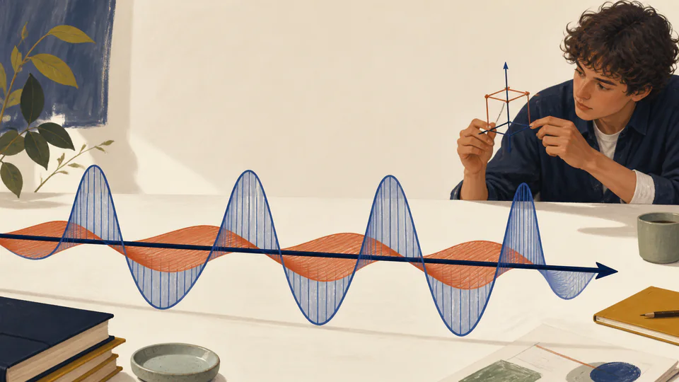
Editorial illustration of perpendicular electric and magnetic field ribbons traveling together through open space
The electric and magnetic components oscillate in phase, perpendicular to each other and to propagation.
Electric and magnetic field versus positionThe magnetic trace is normalized for visual comparison, while the ledger preserves tesla values and the E0/B0 = c relation.
Field sample ledgerCurrent unrounded calculation path
Use the entered frequency, amplitude, time, and phase to evaluate both transverse components at identical positions.
SamplePosition x (m)Electric field Ey (V/m)Magnetic field Bz (T)Ey/Bz ratio

DETAILED CALCULATION PROCESS

Formula, units, default substitution, and reconciliation

1. Governing relation

E_y = E0 cos(kx - omega t + phi); B_z = (E0/c) cos(kx - omega t + phi); lambda = c/f; <S> = 0.5 c epsilon0 E0^2

A monochromatic plane wave uses one phase for both transverse fields. Frequency fixes wavelength, E0 fixes B0 through c, and the selected time translates the spatial phase without changing amplitude.

2. Symbols and default basis

SymbolMeaningUnitDefault basis
E0Peak electric-field amplitudeV/m10 V/m
B0Peak magnetic-field amplitudeTE0/c
fWave frequencyHz100 MHz
lambdaVacuum wavelengthmc/f
omegaAngular frequencyrad/s2 pi f
kWave numberrad/m2 pi/lambda
phi, tPhase offset and snapshot timerad; s0 deg; 0 ns

3. Unit and sign normalization

  • Megahertz are multiplied by 1e6 before computing wavelength or angular frequency.
  • Degrees are multiplied by pi/180 before entering the cosine.
  • Nanoseconds are multiplied by 1e-9; magnetic values remain in tesla even when normalized on the canvas.

4. Current numerical substitution

    5. Independent reconciliation

    HOW TO USE THIS CALCULATOR

    Five steps from physical inputs to a defensible result

    1. Choose the monochromatic frequency whose vacuum wavelength you want to inspect.
    2. Enter the peak electric-field amplitude, or zero for the valid zero-field boundary.
    3. Set phase offset to define the field value at the origin.
    4. Move snapshot time to see propagation as a phase shift while keeping wavelength fixed.
    5. Read exact field samples in the ledger; use the canvas for pattern recognition, not precise extraction.

    PHYSICS FOUNDATIONS FOR THIS MODEL

    Concepts that control this specific calculation

    A graph needs a declared independent variable
    This page puts position x on the horizontal axis while holding time fixed.
    Fields are transverse
    E_y, B_z, and propagation along x are mutually perpendicular in this ideal wave.
    The components are in phase
    Their maxima and zero crossings occur at the same x and t in vacuum.
    Frequency fixes spatial period
    One wavelength is the distance over which phase advances by 2 pi at a fixed instant.
    Different units require honest scaling
    V/m and tesla differ by c, so the canvas normalizes B only for visibility and the table reports actual values.

    DEEP ANALYSIS 1

    Time shifts phase, not wavelength

    Increasing t translates the displayed pattern in the propagation direction; it does not stretch the spatial period.

    DEEP ANALYSIS 2

    Mean intensity is not the instantaneous field curve

    The Poynting-vector average depends on E0 squared. Negative field values indicate direction, not negative transported energy.

    DEEP ANALYSIS 3

    Plane-wave assumptions fail near sources

    Reactive near fields, curved wavefronts, finite beams, polarization mixtures, and material boundaries require Maxwell solutions beyond this graph.

    RESULT INTERPRETATION

    What the current output does and does not decide

    A zero electric amplitude leaves wavelength and phase coordinates defined but makes both fields and intensity zero. This is a useful wiring boundary for the graph.

    If the visual E and normalized B traces do not overlap, the implementation has broken the vacuum plane-wave phase relation; the exact ledger provides the check.

    REAL USE CASES

    Two decisions with different boundary conditions

    100 MHz teaching snapshot

    A two-wavelength span makes nodes, peaks, and the E/B phase relation visible while the sample ledger ties each plotted location to SI values.

    Phase-referenced bench comparison

    A field probe record uses a known phase reference. Adjusting phi and snapshot time distinguishes a coordinate choice from a change in frequency or amplitude.

    EVIDENCE AND DATA QUALITY

    What to retain with the exported result

    Retain the stated propagation axis, polarization convention, amplitude definition (peak versus RMS), frequency reference, time origin, phase reference, and whether vacuum propagation is a justified approximation.

    LIMITS AND EXCLUSIONS

    Where this physical model stops

    • The wave is monochromatic, sinusoidal, linearly polarized, and planar.
    • Propagation is in vacuum with no attenuation, dispersion, reflection, or boundary.
    • The electric input is peak amplitude, not RMS.
    • The canvas normalizes magnetic amplitude solely for visibility; the ledger retains tesla.
    • Near-field antennas, pulses, broadband spectra, standing waves, and material media are outside scope.

    TERMS USED HERE

    Six terms that keep the calculation unambiguous

    Plane wave
    Ideal wave with constant phase across each plane normal to propagation.
    Polarization
    Orientation and evolution of the electric-field vector.
    Wave number
    Spatial angular frequency k = 2 pi/lambda.
    Angular frequency
    Temporal angular frequency omega = 2 pi f.
    Phase
    Dimensionless argument locating a point within an oscillation.
    Poynting vector
    Electromagnetic energy-flux vector E cross H.

    RELIABLE SOURCES

    References supporting the equation and units

    FREQUENTLY ASKED QUESTIONS

    Questions specific to this calculation

    Is the horizontal axis time?

    No. It is position at one selected time; changing time shifts the snapshot.

    Why is magnetic field normalized on the graph?

    B is smaller than E by c in SI units, so a shared raw vertical scale would hide it. Exact tesla values remain in the table.

    Can electric amplitude be zero?

    Yes. It creates the valid zero-field boundary while preserving frequency and wavelength.

    Does a negative field mean negative energy?

    No. It means the vector component points opposite the chosen axis; mean energy flow remains based on squared amplitude.

    Can this show a standing wave?

    No. A standing wave needs at least two counter-propagating components and different node behavior.

    Does this model radio propagation loss?

    No. Amplitude is constant with x; use a link-budget scenario for free-space spreading.

    IMPORTANT BOUNDARY

    Use the result as analysis, not certification

    This ideal field snapshot is for physics analysis and education, not antenna certification, EMC compliance, exposure assessment, or field-probe calibration.