Physics and mechanics
Sound Wave Graph Calculator
Plot a real input-driven sound-pressure snapshot along distance, including wavelength, propagation delay, phase, and exponential level attenuation.
CURRENT MODEL
Define the traveling wave and the spatial snapshot
Acoustics students, measurement planners, educators, and audio engineers who need to see how phase and amplitude evolve along a one-dimensional path.
Decision supportedChoose spatial sampling and measurement positions by seeing the actual wavelength, delay, phase, and attenuated pressure generated by the entered conditions.
LIVE PRESSURE-PATH GRAPH
Current pressure snapshot and attenuation envelope
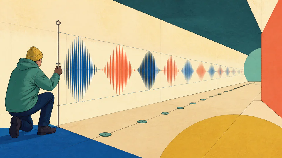
The chart is calculated from 41 positions using the entered frequency, speed, RMS pressure, attenuation, path, time, and starting phase; no decorative data is used.
| Position | RMS envelope (Pa) | Instantaneous pressure (Pa) | Phase (deg) |
|---|
How to use
Freeze one traveling wave at a declared instant
- Enter a positive single frequency and a sound speed for the uniform medium.
- Enter non-negative starting RMS pressure at x = 0 and a non-negative amplitude loss in dB per metre.
- Set the positive path length over which the model will calculate 41 evenly spaced positions.
- Choose snapshot time in milliseconds and starting phase in degrees; changing either shifts phase but not the RMS envelope.
- Compare wavelength with path length to see how many cycles fit in the current spatial window.
- Use the five-row sample ledger and endpoint envelope reconciliation before exporting the graph case.
Spatial graph fundamentals
Six ideas behind the plotted curve
- Spatial snapshot
- Pressure at many positions evaluated at one common time.
- Instantaneous pressure
- Signed deviation from ambient, including compression and rarefaction.
- RMS envelope
- Non-negative local effective amplitude before conversion to peak.
- Phase progression
- Spatial phase decreases by kx for the chosen propagation direction.
- Propagation delay
- Path length divided by sound speed, independent of snapshot phase.
- Amplitude loss
- A pressure-level reduction converted with 10 to the power of minus loss over 20.
Calculation method
Construct phase and envelope independently, then combine them
The model resolves wavelength, period, omega, and k from frequency and sound speed. At each of 41 positions it calculates RMS envelope from the cumulative dB loss, converts RMS to peak with sqrt(2), and evaluates the cosine phase at the entered snapshot time.
Separating envelope from phase is essential: attenuation changes amplitude with distance, while frequency, wave speed, time, and starting phase determine where compressions and rarefactions appear.
Pressure dB conversion
Because attenuation is entered as an amplitude-level loss, pressure ratio uses 20 log10. Using a power-ratio divisor of 10 would exaggerate amplitude decay.
Snapshot versus trace
A microphone time trace holds position fixed and varies time. This graph holds time fixed and varies position, so its horizontal axis must remain metres.
Sampling adequacy
Forty intervals may undersample a path containing many wavelengths. Use the graph for interpretation and a denser solver for numerical extrema or phase-sensitive design.
Missing propagation effects
Constant dB/m decay does not create reflections, diffraction, refraction, interference, geometric spreading, or frequency-dependent atmospheric absorption.
Detailed calculation process
Symbols, current substitution, intermediate quantities, and reconciliation
lambda = c/f; p_rms(x) = p_rms,0 10^(-alpha x/20); p(x,t) = sqrt(2) p_rms(x) cos(2 pi f t - 2 pi x/lambda + phi)The curve uses 41 evenly spaced samples across the entered path and retains full precision. Labels adapt to the pressure scale so small amplitudes remain visible.
| Symbol | Meaning | Default | Unit |
|---|---|---|---|
| f | Single wave frequency | 500 | Hz |
| c | Sound phase speed | 343 | m/s |
| p_rms,0 | Starting RMS pressure at x = 0 | 1 | Pa |
| alpha | Pressure-level attenuation rate | 0.5 | dB/m |
| L | Plotted path length | 3 | m |
| t | Snapshot time | 1 | ms |
| phi | Starting phase | 0 | deg |
| p(x,t) | Instantaneous acoustic pressure | calculated | Pa |
Waiting for valid inputs.
Interpretation
Read the envelope and waveform as different evidence
The upper and lower envelopes show allowable peak magnitude at each position. The oscillating line shows one instantaneous realization inside those bounds. Changing snapshot time moves the oscillation while leaving end RMS pressure and total span attenuation unchanged.
Evidence and measurement
Preserve phase reference and attenuation provenance
Record how frequency, speed, and starting pressure were obtained, the x = 0 reference plane, propagation direction, clock and phase convention, microphone calibration, and whether the dB/m rate came from measured amplitude ratios or an applicable source. Retain raw spatial or time records when fitting attenuation.
Scope and limitations
What this one-dimensional snapshot excludes
- Spherical or cylindrical geometric spreading
- Reflections, room modes, interference, diffraction, and barriers
- Dispersion and frequency-dependent attenuation
- Broadband signals, impulses, modulation, and stochastic noise
- Vector particle velocity and reactive near fields
- Exposure compliance, structural response, or propagation certification
A single-frequency progressive plane wave travels in a uniform nondispersive medium. Attenuation is a constant amplitude-level loss in dB per metre and reflections are excluded.
Key terminology
Pressure-graph glossary
- Envelope
- Curve bounding the position-dependent peak pressure magnitude.
- Snapshot time
- Single instant at which every spatial sample is evaluated.
- Phase offset
- Declared cycle position at x = 0 and t = 0.
- Attenuation
- Reduction of wave amplitude with propagation distance.
- Compression
- Positive acoustic pressure relative to ambient.
- Rarefaction
- Negative acoustic pressure relative to ambient.
- Propagation delay
- Travel time from the reference plane to the endpoint.
- Spatial sampling
- Discrete positions at which the continuous model is evaluated.
Practical cases
Two graph-reading decisions with different failure modes
Microphone spacing for a tone
A lab plots a 500 Hz tone across a three-metre test path to choose positions that are not accidentally near the same phase. Reflections are measured separately because they would reshape the real field.
Attenuated inspection signal
An engineer enters a measured amplitude-loss rate and changes path length to estimate endpoint RMS pressure and travel delay. The graph helps plan sensor dynamic range, while the full broadband pulse needs a dispersive model.
Important note
A smooth curve is still an idealized propagation model
The graph is generated entirely from current inputs, but visual precision does not prove the assumptions. Retain the unrounded sample data and compare against calibrated measurements before making phase-sensitive decisions.
Frequently asked questions
Is the plotted curve pressure versus time?
No. It is a spatial snapshot: every point shows instantaneous pressure at a different position but at the same entered time. Changing snapshot time advances the phase everywhere.
Why can instantaneous pressure be negative?
Acoustic pressure is the deviation from ambient pressure. Negative portions represent rarefaction, while positive portions represent compression; RMS amplitude remains non-negative.
Why does attenuation use division by 20 rather than 10?
The entered loss is a pressure-amplitude level. Pressure ratios use 20 log10, so recovering the amplitude multiplier uses 10^(-loss/20). Power ratios would use 10 log10.
Does the curve include spherical spreading?
No. It is a one-dimensional plane-wave model with only the entered dB-per-metre decay. Geometric spreading, barriers, atmospheric frequency dependence, and room reflections need separate models.
What happens when starting RMS pressure is zero?
The envelope and every instantaneous sample are exactly zero, while wavelength and travel delay remain defined. The graph becomes a flat zero-pressure line.
How many points does the calculator draw?
It calculates 41 evenly spaced positions, including both endpoints. That is sufficient for an explanatory live view but not a substitute for a high-resolution numerical propagation solver.
Authority and follow-on work
Reliable sources and related calculators
- OpenStax — Speed of Sound, Frequency, and WavelengthSupports wavelength, speed, frequency, and propagation-delay relationships.
- MIT OCW — Chapter 13 AcousticsSupports sinusoidal plane-wave pressure, phase, wavenumber, and RMS notation.
- FHWA — Fundamentals and Abatement of Highway Traffic NoiseProvides practical sound-pressure-level and decibel-ratio context.
Related calculators
Continue with a distinct physics question without silently changing the model boundary.