Physics and mechanics
Electric Field Rate Calculator
Calculate the component and magnitude of the average change in a measured two-dimensional electric-field vector between two timestamps, while keeping vector rate distinct from field-magnitude rate.
CURRENT MODEL
Enter the declared electric-field case
EMC technicians, field-mapping teams, and physics students comparing two time-stamped planar electric-field readings.
Decision supportedDecide whether the measured field changed materially over the declared sample interval and identify which component drove that finite change.
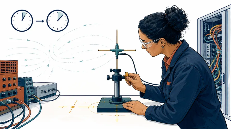
SUBJECT DECISION ILLUSTRATION
The same probe position at two timestamps
The static scene explains the measurement discipline behind the calculation; exact current values remain in the live result cards and ledger.
| Quantity | Symbol / expression | Current value | Unit | Interpretation |
|---|
How to use
Compare two field vectors without losing their measurement context
- Freeze one Cartesian axis convention and record how the probe's x and y channels align with the apparatus.
- Enter the two signed component readings from the same spatial point, calibration state, range, bandwidth, and averaging mode.
- Use timestamps from the acquisition record to enter a strictly positive elapsed interval in milliseconds.
- Read the component rates first to identify whether x, y, or both channels drove the change.
- Compare vector-rate magnitude with field-magnitude rate; disagreement indicates that rotation contributes to the measured change.
- Retain the raw samples and sampling metadata before treating the finite difference as evidence of a transient event.
Rate fundamentals
Five distinctions that keep a two-sample rate honest
- Field vector
- Electric field has magnitude and direction, so signed components must be subtracted in one coordinate frame.
- Finite difference
- Two samples determine one interval-average change; they do not reveal what happened between timestamps.
- Vector-rate norm
- The norm combines component changes and remains nonnegative even when individual rates are negative.
- Magnitude rate
- Change in |E| ignores pure rotation and therefore answers a different question from |Delta E/Delta t|.
- Sampling interval
- Shorter intervals amplify the same measured difference into a larger rate and can magnify timing or noise errors.
Calculation method
Subtract components, normalize by one interval, then reconcile the norms
The calculator converts milliseconds to seconds once, subtracts initial components from final components, and divides both differences by that same interval. It then takes the Euclidean norm of the rate vector and independently computes the change in the two field magnitudes.
This method intentionally reports an average secant rate. Estimating an instantaneous derivative would require more samples, a stated filter or fit, and uncertainty treatment appropriate to the instrument bandwidth.
Rotation with little magnitude change
A field can swing from one direction to another while keeping nearly the same norm. Component rates and vector-rate magnitude expose that motion even when Delta|E| is near zero.
Noise divided by a short interval
Probe noise or timestamp quantization becomes a rate after division by Delta t. A numerically large result can therefore reflect metrology limits rather than a physical transient.
Spatial movement masquerading as time change
If the probe moved through a nonuniform field, the difference mixes spatial gradient with temporal evolution. This page cannot separate those effects from two readings alone.
Detailed calculation process
Symbols, current substitution, intermediate quantities, and reconciliation
E_rate,avg=(E_2-E_1)/Delta tAll component differences and norms use unrounded SI values; display formatting occurs after the scalar and vector reconciliations.
| Symbol | Meaning | Default | Unit |
|---|---|---|---|
| E_1x | Initial x-component | 120 | V/m |
| E_1y | Initial y-component | -40 | V/m |
| E_2x | Final x-component | 180 | V/m |
| E_2y | Final y-component | 20 | V/m |
| Delta t | Elapsed sample interval | 50 ms = 0.05 s | s |
| R_E | Average field-vector rate | calculated | V/(m s) |
| R_|E| | Rate of field-magnitude change | calculated | V/(m s) |
Waiting for valid inputs.
Result interpretation
Read direction, magnitude, and scalar change as separate evidence
A large positive x rate means the signed x-component increased, not necessarily that the total field strengthened. A zero vector rate means both entered vectors match exactly. A large vector-rate magnitude paired with a small magnitude rate points to directional rotation, while similar values suggest predominantly radial strengthening or weakening in component space.
Evidence to retain
Preserve the acquisition chain behind both timestamps
Keep the raw channel values, timestamp precision, probe serial number, calibration date, axis sketch, physical coordinates, frequency response, bandwidth, averaging window, range setting, temperature, nearby switching state, and any probe repositioning. A copied rate without those facts is not reproducible.
Scope and limitations
What two samples cannot establish
- No instantaneous derivative, waveform peak, rise time, or spectral content
- No correction for sensor lag, anti-alias filtering, clipping, or noise floor
- No separation of temporal variation from probe motion through a spatial gradient
- No z-component, coordinate rotation, or uncertainty propagation
- No exposure, EMC compliance, insulation, or safety-limit decision
- No causal attribution to a nearby source or switching event
Two field vectors expressed in one fixed Cartesian frame, measured at the same spatial point and under comparable sensor conditions. The output is an average finite difference, not an instantaneous derivative.
Key terminology
Field-rate glossary
- Finite difference
- A change between two discrete samples divided by their separation.
- Secant rate
- An interval-average slope rather than the tangent slope at one instant.
- Vector norm
- The nonnegative magnitude formed from orthogonal component values.
- Coordinate frame
- The fixed axes that give each signed field component its meaning.
- Probe bandwidth
- The frequency range over which the sensor can follow field changes reliably.
- Timestamp quantization
- The finite time resolution that limits how precisely the sample interval is known.
Practical cases
Two different reasons to compute the interval rate
Switching-cabinet repeatability check
An EMC technician compares vectors immediately before and after a controlled relay action at a fixed probe fixture. A dominant y-component rate leads the team to inspect conductor orientation and repeat the acquisition with a higher sample rate.
Outdoor mapping false alarm
A survey team sees a large two-sample rate but discovers the handheld probe moved several centimetres near an energized cable. The rate is retained as a mixed spatial-temporal observation, not reported as a field transient.
Important note
A computed rate is not an instrument-performance or safety verdict
Review calibration, bandwidth, sampling, uncertainty, spatial stability, and the governing measurement procedure before using this finite difference in engineering or exposure decisions.
Frequently asked questions
Is this the instantaneous time derivative of the electric field?
No. It is the average finite difference between two samples. An instantaneous derivative requires a sufficiently resolved time series and a defensible differentiation method.
Why can vector-rate magnitude differ from the rate of field magnitude?
The field can rotate while changing little in magnitude. The norm of the component-rate vector captures directional change; Delta|E|/Delta t captures only scalar magnitude change.
What if both readings are identical?
The component and vector rates are exactly zero. A direction is not assigned because a zero vector has no unique angle.
Can readings from different probe orientations be compared directly?
Not without rotating them into one common coordinate frame. Treating instrument axes as identical when they moved creates a false field change.
Does a large rate prove a transient hazard?
No. Probe bandwidth, averaging, calibration, spatial movement, interference, and the applicable exposure or equipment standard must be reviewed separately.
Why is the elapsed time entered in milliseconds?
Many transient measurements are timestamped in milliseconds; the calculator converts the interval once to seconds so the output remains V/(m s).
Authority and follow-on work
Reliable sources and related calculators
- OpenStax Calculus Volume 3 - Vector-Valued DerivativesDefines vector derivatives component by component and interprets them as rates of change.
- OpenStax University Physics - Electric FieldDefines electric field as a vector and states its N/C unit and direction convention.
- NIST SP 811 - Guide for the Use of SISupports coherent SI quantity and unit reporting.
Related calculators
Continue with a genuinely different electric-field question without silently changing this page's assumptions.