PH

Physics calculator

Friction Trajectory Calculator

Model a one-dimensional friction trajectory with a static-friction start gate, kinetic-friction motion, exact zero-speed events, and live position and velocity history.

Piecewise motion under dry friction

Will the object stay at rest, stop within the interval, reverse, or still be sliding at the requested horizon?

Follow an object along a signed axis on an incline. The model first decides whether static friction can hold, then applies kinetic friction during each sliding segment and rechecks the static gate whenever velocity reaches zero.

Designed for: For students, lab teams, and preliminary design checks that need the full time history rather than a single stopping-distance number.

Position at duration -
Velocity at duration -
First stop time -
Position at first stop -
Normal force -
Final motion state -

LIVE MODEL OUTPUT

Current trajectory samples

Time-ordered state produced from the current inputs and every zero-speed event.
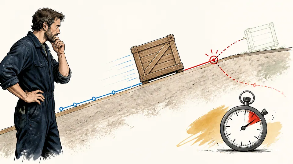
Current visualization updates with every valid input change.
Editorial illustration of a crate tracing a changing motion path down a textured ramp while an engineer marks the stop point.
A trajectory question is about what happens before and after the stop, not only the final distance.
Current trajectory samplesExact values from the current model state
Time-ordered state produced from the current inputs and every zero-speed event.
Time (s)Friction statePosition (m)Velocity (m/s)Acceleration (m/s^2)

CURRENT CALCULATION PROCESS

Formula, units, substitution, intermediate quantities, and check

N = m x g x cos(theta); D = F - m x g x sin(theta); |D| <= mu_s x N holds at rest; a = [D - sign(v) x mu_k x N] / m while sliding

The axis is fixed to the plane. Motion is integrated in constant-acceleration pieces. If a piece would cross zero velocity, the exact crossing time is solved first; the remaining time is then evaluated under the static-friction rule before any reverse motion begins.

Symbols, meanings, units, and defaults for this page model
SymbolMeaningUnitDefault
mTranslating masskg12
v0Initial signed velocitym/s8
mu_sStatic friction coefficientunitless0.42
mu_kKinetic friction coefficientunitless0.30
thetaIncline angle, positive upslopedeg0
FSigned applied force along planeN0
TModeled durations5
dtOutput sample intervals0.25

Conversions and rounding: Angles are converted from degrees to radians for sin and cos. All other defaults are already SI. Display values are rounded, but event times and integration retain full floating-point precision.

    HOW TO USE

    Build a defensible friction trajectory

    1. Choose a signed axis and enter velocity and force with that same direction convention.
    2. Enter static and kinetic coefficients from the same contact pair and surface condition.
    3. Set the incline angle; use zero for a horizontal surface and keep applied force parallel to the plane.
    4. Choose a duration long enough to include the possible stop and a sample interval fine enough to inspect it.
    5. Read the state table and chart together, then use the first-stop result only if the model actually reaches zero velocity.

    SUBJECT FUNDAMENTALS

    What determines the trajectory

    Static friction is a response
    At rest, friction takes the magnitude needed for equilibrium up to mu_s x N; it is not automatically equal to its maximum.
    Kinetic friction has a direction
    During sliding, mu_k x N acts opposite the instantaneous velocity, so its sign can change after a reversal.
    The incline changes two terms
    Gravity contributes m x g x sin(theta) along the plane and leaves m x g x cos(theta) to create normal force.
    Stopping is an event
    A time step must not jump through zero velocity. The model solves the crossing exactly and then tests static friction again.
    Position can remain nonzero
    A stopped object holds its accumulated displacement; velocity goes to zero but the earlier travel is not erased.
    Coefficients describe conditions
    Dry, clean, contaminated, hot, or polished interfaces can have materially different coefficients even for the same materials.

    RESULT INTERPRETATION

    Read the path as a sequence of regimes

    Static hold

    Zero velocity with a static-hold label means the required friction is within capacity, not that mu_s x N is fully mobilized.

    Sliding label

    Upslope or downslope describes velocity direction. Acceleration may point the other way while the object slows.

    First stop

    The first stop is a diagnostic event. Later motion can occur if the static gate fails after that event.

    DEEPER ANALYSIS

    Three trajectory decisions hidden by one-line formulas

    Stopping versus reversing

    If the non-friction drive is inside the static limit when speed reaches zero, the object stays there. If it exceeds the limit, a new kinetic segment starts in the drive direction.

    Sampling versus event precision

    The table is sampled at dt, but stop time is not rounded to that grid. This prevents a coarse reporting interval from moving the physical stop point.

    Changing normal load

    This page assumes the applied force is parallel to the plane. A rope angled away from the surface would reduce N and both friction limits; use a force-component model instead.

    WORKED CASES

    Worked motion cases

    Warehouse tote stopping on level flooring

    For m = 12 kg, v0 = 8 m/s, mu_k = 0.30, and no applied force, acceleration is about -2.942 m/s^2. The tote stops near 2.72 s and 10.88 m, then static friction holds because the horizontal drive is zero.

    Cart released on a steep ramp

    With v0 = 0, the model first compares m x g x sin(theta) with mu_s x m x g x cos(theta). If tan(theta) exceeds mu_s, the cart starts downslope; entering a small nonzero velocity is not required to trigger motion.

    ASSUMPTIONS

    Model assumptions to record

    • One-dimensional translation along a rigid plane.
    • Constant mass, incline, gravity, applied force, and friction coefficients.
    • No aerodynamic drag, rolling resistance, wheel inertia, deformation, or speed-dependent friction.
    • Continuous contact with no applied force component normal to the plane.
    • mu_s >= mu_k so the launch rule is mechanically coherent for this simplified dry-friction model.

    TECHNICAL LANGUAGE

    Trajectory-specific terms

    Static limit
    The largest friction magnitude available while the contact has no relative sliding.
    Kinetic segment
    A time interval with nonzero sliding velocity and a fixed friction direction.
    Drive force
    The signed sum of applied and along-plane gravity forces before friction is included.
    Zero-speed event
    The exact instant a sliding solution reaches v = 0 and must be reclassified.
    Stopping distance
    Position accumulated from the starting point to the first zero-speed event.
    Signed axis
    A declared positive direction that gives force, velocity, acceleration, and position consistent signs.

    EVIDENCE AND DATA LINEAGE

    Evidence to preserve with a result

    Record the contact materials and condition, how mu_s and mu_k were obtained, incline measurement, force direction, mass, time horizon, sample interval, and the exported table. A coefficient copied from a generic table is an assumption, not a test result for the actual interface.

    LIMITS AND EXCLUSIONS

    Where this trajectory should not be used

    • Do not use for rolling tires, bearings, lubricated contacts, or stick-slip systems without a validated friction law.
    • Do not use after contact loss, impacts, or geometry changes.
    • The model does not include speed-dependent drag or a force that varies with time or position.
    • A result near a friction threshold is sensitive to coefficient uncertainty and surface contamination.
    • This is a deterministic nominal path, not a confidence interval or safety certification.

    RELIABLE SOURCES

    Primary references and stated use

    FREQUENTLY ASKED QUESTIONS

    Questions about friction paths and stopping events

    Why can the stop time fall between table rows?

    The solver locates the exact zero of v within a constant-acceleration segment. The sample interval controls reporting density, not event accuracy.

    Why is static friction checked after a stop?

    Kinetic friction no longer applies once sliding velocity is zero. The object can remain stopped only if static friction can balance the drive.

    Can I enter a negative incline?

    Yes. A negative angle makes gravity act toward the positive axis under the stated sign convention.

    Why must mu_s be at least mu_k here?

    The simplified launch-and-slide rule assumes a larger or equal breakaway capacity. If your measured interface violates that relation, it needs a more specific friction model.

    Does a zero final velocity prove the object never moved?

    No. Check end position and the trajectory table; the object may have traveled and then stopped.

    Can I model a force pulse?

    Not on this page. Applied force is constant. Split the motion into separately documented intervals or use a time-varying dynamics solver.

    IMPORTANT NOTE

    Engineering and laboratory use note

    This calculator implements an idealized Coulomb-friction model for education and preliminary analysis. Verify coefficients and forces experimentally before relying on the result for safety, braking, lifting, transport, or equipment design.