Physics and mechanics
Heat Transfer Graph Calculator
Plot temperature difference, instantaneous heat-transfer rate, and cumulative energy versus time from a real lumped-capacitance model and current inputs.
CURRENT MODEL
Enter the declared thermal case
Thermal-test, product, and process users screening how a small thermally uniform body approaches a constant ambient temperature.
Decision supportedEstimate the time scale, end temperature, rate decay, and accumulated energy for a lumped body before choosing a test duration or a higher-fidelity transient model.
LIVE THERMAL ANALYSIS
Temperature, rate, and cumulative energy over time
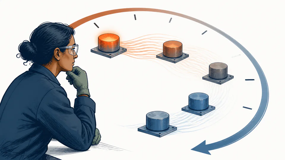
All three live curves are generated from the current lumped-capacitance samples. The table is the accessible exact-value counterpart to the plot.
| Time (min) | Body temperature (deg C) | Delta T (K) | Rate (W) | Cumulative energy (kJ) |
|---|
How to use
Build a transient case that can justify a graph
- Enter the body's uniform initial temperature and the constant bulk ambient temperature.
- Use an effective heat-transfer coefficient for the actual flow and surface condition.
- Enter exposed area, total thermally active mass, and average specific heat over the interval.
- Choose the graph duration; zero minutes is a valid initial-state boundary.
- Confirm lumped-capacitance applicability independently, including the internal-to-external resistance relationship.
- Compare the end card with the final table row and read cumulative energy as stored-energy change, not a separate fitted curve.
Transient fundamentals
Five ideas explain the curve shape
- Lumped body
- The model assigns one uniform temperature to the entire body.
- Thermal capacitance
- m c stores sensible energy for each kelvin of body-temperature change.
- Conductance hA
- The external path that transfers energy for each kelvin of difference.
- Time constant
- m c/(hA), the characteristic time for exponential response.
- Instantaneous rate
- hA times the remaining body-to-ambient temperature difference.
- Cumulative energy
- The integral of rate, reconciled to m c times the body temperature change.
Calculation method
Solve the first-order energy balance at thirteen times
The model balances stored sensible energy m c dT/dt against convection hA(T minus T_inf). With constant properties and ambient temperature, the difference decays as exp(-t/tau). Thirteen evenly spaced samples drive the plotted lines and exact table.
Signed rate is positive when the body is hotter than ambient and negative during heating from a warmer ambient. Cumulative energy follows the same convention as energy leaving the body in the current implementation.
Biot-number gate
The equation does not prove internal uniformity. Characteristic length, body conductivity, and h are needed to evaluate whether spatial gradients are small enough.
Property drift
Natural-convection h and specific heat can change with temperature. A constant-coefficient curve is a screening model, not evidence that real decay is exactly exponential.
Curve normalization
At one tau the difference falls to 36.8%; at three tau it is about 5%. These are model landmarks, not automatic test-duration requirements.
Energy-rate reconciliation
The area under the rate curve must equal the change in stored sensible energy. That conservation check catches graph scaling or time-unit errors.
Detailed calculation process
Symbols, current substitution, intermediate quantities, and reconciliation
T(t) = T_inf + (T_0 - T_inf) exp[-hAt/(mc)]; qdot(t) = hA[T(t)-T_inf]The exponential model uses seconds and unrounded values. Display uses two decimals for temperature and time, 0.1 W for rates, and 0.1 kJ for cumulative energy; the plot uses the unrounded series.
| Symbol | Meaning | Default | Unit |
|---|---|---|---|
| T_0 / T_inf | Initial body / constant ambient temperature | 90 / 20 | deg C |
| h | External heat-transfer coefficient | 8 | W/(m2 K) |
| A | Exposed area | 0.5 | m2 |
| m | Thermally active mass | 20 | kg |
| c | Specific heat capacity | 500 | J/(kg K) |
| tau | m c/(hA) | 41.67 | min |
| t | Elapsed graph time | 0 to 120 | min |
Waiting for valid inputs.
Evidence and measurement
Retain the thermal test boundary
Save sensor locations, calibration, sampling interval, body mass, exposed area, material conductivity, specific heat source, airflow condition, and ambient stability. If fitting h from data, preserve the fit interval and residuals instead of treating the coefficient as a universal property.
Scope and limitations
What the exponential graph excludes
- Spatial temperature gradients and multidimensional conduction
- Changing ambient temperature, h, area, or heat capacity
- Radiation, evaporation, phase change, and internal generation
- Contact resistance to fixtures or mixed boundary conditions
- Sensor lag and control-system dynamics
- Biot-number calculation, safety limits, and material damage criteria
Uniform body temperature; constant ambient temperature, h, area, mass, and specific heat; no internal generation, radiation, phase change, or spatial gradients. The user must independently confirm that lumped capacitance is appropriate, commonly with a sufficiently small Biot number.
Key terminology
Transient-curve glossary
- Lumped capacitance
- A model with one spatially uniform body temperature.
- Time constant
- The m c/(hA) response time in this first-order model.
- Biot number
- A dimensionless comparison of internal conduction and surface transfer resistance.
- Ambient temperature
- The bulk environment value assumed constant here.
- Thermal capacitance
- The body's m c energy storage per kelvin.
- Decay factor
- exp(-t/tau), the fraction of initial temperature difference remaining.
- Instantaneous rate
- The heat-transfer power at one time.
- Cumulative energy
- The time integral of the rate through the current endpoint.
Practical cases
Two graph decisions with different failure modes
Cooling a small metal test coupon
A lab estimates when a high-conductivity coupon approaches room temperature. The graph supports sampling duration after a low-Biot check; sensor contact and radiation remain test uncertainties.
Heating a packaged product
A process team enters ambient hotter than the product, producing negative signed cooling-out rate and rising temperature. Thick packaging or internal phase changes invalidate the one-temperature assumption.
Important note
A smooth curve can still be the wrong model
Visual fit alone does not establish uniform internal temperature or constant h. Check residual patterns, internal sensors, and Biot-number evidence before using the curve for product safety, sterilization, or damage limits.
Frequently asked questions
Why is the curve exponential?
With constant hA and heat capacity mc, the heat rate is proportional to the remaining temperature difference. The same fraction of that difference decays during each time constant.
What does one time constant mean?
After one time constant, the temperature difference is exp(-1), about 36.8%, of its initial value. The body has completed about 63.2% of the modeled approach to ambient.
Can I use this for a thick wall or large object?
Only if internal temperature gradients are negligible. If the Biot number or measurements show spatial gradients, use a transient conduction model with geometry and material conductivity.
Why does the heat-transfer rate fall over time?
The model holds h and area constant while the body approaches ambient, so the driving temperature difference shrinks. Rate equals hA times that instantaneous difference.
How is cumulative energy checked?
The time integral of heat rate equals the modeled change in stored sensible energy, mc times the initial temperature minus the current temperature, with sign preserved.
Does this graph include radiation or evaporative cooling?
No. Those mechanisms can create nonlinear, property-dependent behavior that a constant effective coefficient may not represent. Add them in a more complete energy balance when material.
Authority and follow-on work
Reliable sources and related calculators
- DOE recommended practices for thermal-property testingLumped-capacitance energy balance and applicability discussion.
- U.S. DOE heat-transfer handbookConvection and transient heat-transfer foundations.
- NIST Guide to the SITemperature differences in kelvins and degrees Celsius.
Related calculators
Continue with a distinct heat-transfer question without silently changing the model boundary.