Physics and mechanics
Lens Graph Calculator
Graph signed image distance and magnification across a real-object distance scan for one ideal thin lens, preserving the focal-plane discontinuity and current operating point.
CURRENT MODEL
Enter the declared physical case
Optics students, projection technicians, and bench designers studying how focus and image scale change as a real object moves.
Decision supportedIdentify sensitive object positions, real and virtual branches, and whether a chosen operating point sits too close to the focal-plane asymptote.
LIVE PHYSICAL ANALYSIS
Image-distance and magnification branches
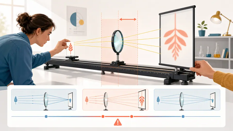
The live two-panel graph marks the current object distance, separates the focal discontinuity, and labels real versus virtual behavior.
| Object distance (cm) | Image distance (cm) | Magnification | Image height (cm) | Image type | Orientation |
|---|
How to use
Scan focus without drawing through the singularity
- Enter the signed focal length from a measured or manufacturer-supported first-order specification.
- Choose a positive real-object distance and height for the highlighted operating point.
- Set scan limits wide enough to expose the real and virtual branches relevant to the bench.
- Read image distance and magnification together; a large focus shift can accompany a modest scale change.
- Inspect the sensitivity value before choosing a mechanical focus tolerance.
- Preserve the focal-plane gap and use ray tracing when thickness, aberration, or field angle matters.
Graph fundamentals
Five features of a thin-lens sweep
- Object-distance axis
- Each horizontal position is a separate real-object placement measured from the principal plane.
- Image-distance branch
- Positive values locate real images behind the lens; negative values locate virtual images on the object side.
- Magnification branch
- The signed image-to-object height ratio changes orientation as well as scale.
- Focal asymptote
- At d_o=f the reciprocal image distance is zero and no finite screen position exists.
- Local sensitivity
- The derivative shows how strongly a small object displacement moves the ideal image plane.
Calculation method
Evaluate one operating point and a consistent sweep
Every graph sample uses d_i=f d_o/(d_o-f), then m=-d_i/d_o and h_i=m h_o. Samples at the focal boundary are marked discontinuous instead of replaced with a large finite number.
The current marker uses exactly the same model as the cards and table. The graph provides shape and sensitivity; the ledger provides exact signed values and image classification.
Near-focus mechanical amplification
When d_o approaches f, the denominator shrinks and millimetres of object movement can demand much larger screen travel. This is a focus-mechanism risk, not extra optical precision.
Virtual and real branches
The branch sign distinguishes a projectable real image from a virtual image that must be viewed through the lens or relayed by another element.
Graph-reading limits
A steep curve can look vertical because of plotting scale, while clipping extreme values can hide the asymptote. Use the exact table before making a tolerance decision.
Detailed calculation process
Symbols, current substitution, intermediate quantities, and reconciliation
d_i(d_o)=f d_o/(d_o-f); m=-d_i/d_o; h_i=m h_oThe sweep and classification use unrounded values; display rounding occurs after the reciprocal check.
| Symbol | Meaning | Default | Unit |
|---|---|---|---|
| f | Signed focal length | 10 | cm |
| d_o | Current real-object distance | 30 | cm |
| d_i | Signed image distance | calculated | cm |
| h_o | Object height | 5 | cm |
| m | Signed magnification | calculated | dimensionless |
| S | Local image-distance sensitivity | calculated | cm/cm |
Waiting for valid inputs.
Evidence to retain
Record what fixes the plotted geometry
Keep lens identity, wavelength, effective focal-length method, principal-plane reference, object and screen coordinates, focus criterion, object depth, temperature, aperture, scan limits, and measurement uncertainty. A catalog focal length alone does not reproduce a measured curve.
Scope and limitations
What the sweep excludes
- No thick-lens principal-plane separation or multi-element transfer matrix
- No spherical or chromatic aberration, distortion, vignetting, diffraction, or depth of field
- No finite object depth or tilted object plane
- No sensor acceptance criterion beyond ideal image height
- No mechanical backlash or focus-position uncertainty
- No safe interpolation across the focal discontinuity
One paraxial thin lens, real object, one surrounding medium, distances from the principal plane, and no aberration or lens thickness.
Key terminology
Focus-curve glossary
- Conjugate distances
- The paired object and image distances linked by the lens equation.
- Principal plane
- The first-order reference plane from which effective conjugate distances are measured.
- Real image
- A converging-ray image that can be intercepted by a screen.
- Virtual image
- An apparent source formed by diverging rays and assigned negative image distance here.
- Asymptote
- A mathematical boundary approached without a finite image-distance value.
- Paraxial
- The small-angle, near-axis regime underlying the thin-lens relation.
Practical cases
Two reasons to inspect the full curve
Projection focus travel
A projector designer scans the expected object movement around a positive focal length and sees that the screen carriage would need excessive travel near focus. The design moves to a longer object distance.
Diverging-lens classroom check
A student enters a negative focal length and confirms the graph has no positive-object asymptote and keeps a virtual upright image. A ray sketch is then used to explain the sign.
Important note
A smooth plotted branch is still an idealization
Do not set production focus tolerances from the derivative alone. Measure the assembled optical path at the working wavelength and include principal-plane uncertainty, aberration, sensor criterion, and mechanical repeatability.
Frequently asked questions
Why does the graph break at the focal length?
At d_o=f the ideal output is collimated and d_i has no finite value. Connecting the two branches would draw a false path through Infinity.
Why is image distance negative on part of the graph?
Under the declared convention, negative d_i is a virtual image on the object side of the lens; it cannot be caught on a screen behind the lens.
What does the sensitivity value mean?
It is the local change in image distance per unit object movement. Its magnitude grows sharply near the focal-plane boundary.
Can a diverging lens create the same asymptote for a real object?
No. With negative focal length and positive real-object distance, d_o-f does not vanish; the image remains virtual in this simple model.
Does the graph include depth of field?
No. Depth of field requires an aperture, circle-of-confusion criterion, sensor geometry, and acceptable blur definition.
Why may a measured curve differ?
Principal-plane location, lens thickness, wavelength, aberrations, object depth, and focus measurement uncertainty can shift the observed relation.
Authority and follow-on work
Reliable sources and related calculators
- OpenStax College Physics 2e - Image Formation by LensesThin-lens equation, magnification, and sign interpretation.
- OpenStax University Physics - Thin LensesWorked conjugate and magnification examples.
- NIST SI Length GuidanceSupports coherent length-unit reporting.
Related calculators
Continue with a distinct physical question without silently changing this page's model boundary.