p

Physics and geometric optics

Mirror Graph Calculator

Graph signed image distance and magnification against real-object distance for a concave or convex spherical mirror.

Object-distance response curve

See where mirror response changes gradually, sharply, or without bound

This page samples the signed spherical-mirror equation across a chosen real-object range. It explicitly breaks a concave curve at the focal singularity instead of drawing a false line through infinity.

Reference image distance-
Reference magnification-
Reference image height-
Sampled finite span-

Current model evidence

Mirror response-curve ledger

Link the highlighted reference result to a domain-aware scan that never bridges a focal asymptote.
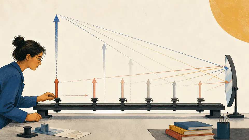
Editorial optical bench showing one object moved through several positions before a concave mirror with changing reflected-image locations
Moving an object by equal distances does not move the image by equal distances, especially near a concave focal point.
Signed image distance and magnification versus object distanceBoth panels share the entered do axis, mark the reference point, and show a focal asymptote when it lies inside a concave scan.
Mirror response-curve ledgerCurrent unrounded calculation path
Link the highlighted reference result to a domain-aware scan that never bridges a focal asymptote.
Curve basisLower / current valueUpper / focal valueDerived valueScope / unit

DETAILED CALCULATION PROCESS

Formula, units, default substitution, and reconciliation

1. Governing relation

di(do) = f do/(do - f); m(do) = -di/do = -f/(do - f)

Assign the signed focal length, sample only positive real-object distances, calculate signed di and m at each sample, insert a gap around a concave focal singularity, and evaluate the reference with the same direct equations.

2. Symbols and default basis

SymbolMeaningUnitDefault basis
doScanned real-object distancecm25 to 120 cm
fSigned focal lengthcm+20 cm for concave
di(do)Signed image-distance responsecmCurve output
m(do)Signed magnification response1Curve output
do,refHighlighted object distancecm60 cm
hoReference object heightcm5 cm

3. Unit and sign normalization

  • Range, focal magnitude, reference distance, and height all use centimetres.
  • Mirror type supplies the focal sign; the focal-magnitude field remains positive.
  • Null graph samples are intentional domain gaps, not zeros or missing calculations.

4. Current numerical substitution

    5. Independent reconciliation

    HOW TO USE THIS CALCULATOR

    Five steps from measured inputs to a defensible result

    1. Choose the mirror type and enter a positive focal magnitude.
    2. Set a positive object-distance interval with the minimum below the maximum.
    3. Place the reference distance inside that interval and away from a concave focal point.
    4. Use the image-distance panel for bench placement and the magnification panel for size and orientation regime.
    5. Inspect the asymptote and exact reference ledger before interpolating any design decision from the curve.

    MIRROR PHYSICS FOUNDATIONS

    Concepts that control this specific model

    The response is hyperbolic
    Both di and m depend on 1/(do-f), so equal object steps do not produce equal image changes.
    A concave focal point divides regimes
    Below f the image is virtual and upright; above f it is real and inverted.
    Convex response has no positive-object singularity
    With f < 0 and do > 0, the denominator do-f stays positive.
    Signed axes retain physical meaning
    Negative image distance and positive magnification identify virtual upright images.
    A plotted sample is not a new formula
    The highlighted point and curve use the same mirror equation; sampling only reveals its behavior over a domain.

    DEEP ANALYSIS 1

    Never connect across infinity

    A straight segment between large positive and negative di values would imply a finite path through the focal point. The visual uses a gap and asymptote marker.

    DEEP ANALYSIS 2

    Graph scaling must not rewrite results

    Extreme near-focus samples can dominate the canvas. Display clipping improves readability, while the exact reference value and ledger retain the unrounded model.

    DEEP ANALYSIS 3

    Sensitivity is encoded by slope

    Near f a small do measurement error can cause a large di change. A steep curve is therefore a warning to quantify tolerances before placing a screen.

    RESULT INTERPRETATION

    What the current output does and does not decide

    The reference cards are exact direct evaluations at do,ref; use the curve to understand nearby behavior rather than reading a low-resolution pixel value.

    The finite sampled span summarizes the selected numerical samples and is not a physical limit on image distance near a singularity.

    REAL USE CASES

    Two decisions with different boundary conditions

    Choosing a stable projection range

    Scanning a concave 20 cm mirror from 25 to 120 cm shows rapid variation near the lower edge and progressively steadier screen positions farther beyond 2f.

    Surveying a convex viewing mirror

    A convex scan remains virtual and upright for every positive object distance, approaching a smaller-magnitude negative image distance as the object moves farther away.

    EVIDENCE AND DATA QUALITY

    What to retain with the exported result

    Retain the selected domain, sample count, focal sign convention, exact reference point, curve-gap rule, object-distance measurement method, and aperture conditions.

    LIMITS AND EXCLUSIONS

    Where this physical model stops

    • Uses 181 explanatory samples rather than adaptive optical ray tracing.
    • Excludes the concave focal singularity from finite graph points.
    • Applies only to paraxial spherical mirrors and one real object.
    • Canvas display clipping does not change exported exact values.
    • Does not model aperture, aberrations, reflectance, diffraction, or uncertainty bands.

    TERMS USED HERE

    Six terms that keep the calculation unambiguous

    Response curve
    Output evaluated across a controlled input domain.
    Asymptote
    Line approached without a finite value at the focal singularity.
    Domain gap
    Intentional break where the finite equation result is undefined.
    Reference point
    Exact current object distance marked on each curve.
    Signed image distance
    Positive for real convergence and negative for a virtual image.
    Sensitivity
    Rate at which an output changes for a small input change.

    RELIABLE SOURCES

    References supporting the equation and units

    FREQUENTLY ASKED QUESTIONS

    Questions specific to this calculation

    Why is there a break in a concave graph?

    At do = f the paraxial image is at infinity, so connecting the two finite branches would be physically false.

    Why must the reference stay inside the range?

    The marker and exact cards are intended to explain the displayed domain; an external reference would not be visible.

    Can the range start below the focal length?

    Yes. That includes the virtual-image branch, provided the graph treats the focal point as a gap.

    Why does the convex curve not cross infinity?

    For f < 0 and do > 0, do-f cannot be zero.

    Is sampled finite span the maximum possible di?

    No. It is only the range among finite samples and grows without bound as a concave sample approaches f.

    Can I infer blur from the graph?

    No. Blur requires aperture and aberration information that the paraxial equation does not contain.

    IMPORTANT BOUNDARY

    Use the result as analysis, not certification

    This sampled paraxial response is an educational and first-order planning aid, not an aberration analysis, tolerance simulation, or optical-design certification.