Physics and mechanics
Sound Wave Scenario Calculator
Compare two free-field sound paths from one measured reference level, including distance spreading, path attenuation, insertion loss, duration, receiver pressure, and sound exposure level.
CURRENT MODEL
Enter the declared physical case
Noise-control engineers, site planners, event technicians, and students comparing two receiver placements or mitigation packages from the same measured source condition.
Decision supportedChoose the lower receiver-level scenario and see whether a duration difference reverses the ranking when sound exposure, rather than instantaneous level, is the relevant quantity.
LIVE PHYSICAL ANALYSIS
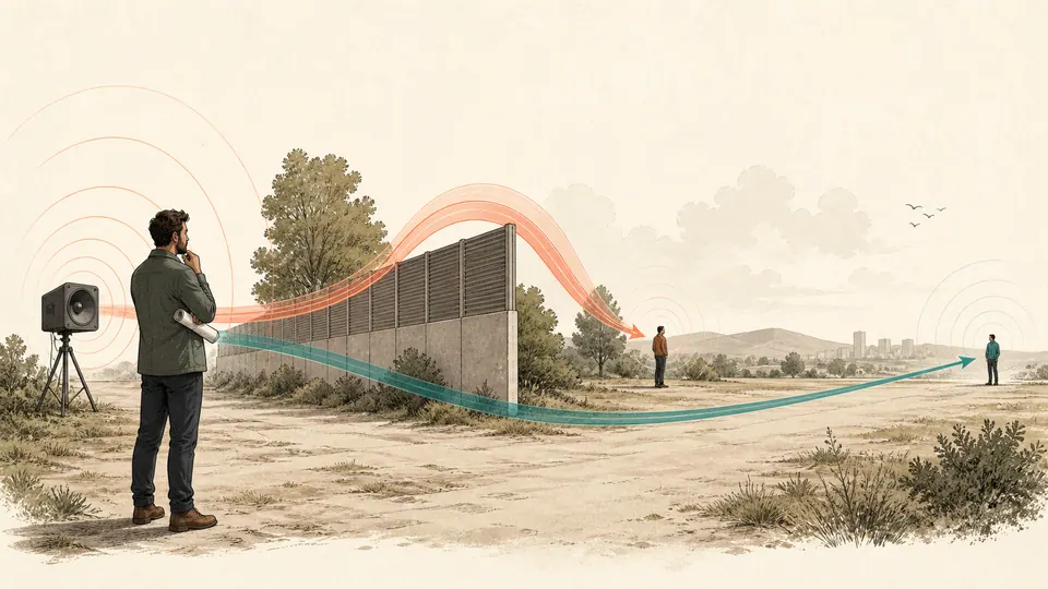
Two complete paths, one reference source
The live bars compare receiver SPL while the annotations preserve distance and insertion-loss assumptions for each path.
| Scenario | Distance (m) | Spreading loss (dB) | Medium loss (dB) | Insertion loss (dB) | Receiver SPL (dB) | Exposure level (dB) |
|---|
How to use
Build two comparable receiver cases
- Record one representative unweighted source level and the exact far-field distance where it was measured.
- Set a common path-attenuation rate only when the same frequency band and atmospheric state apply to both paths.
- Enter Scenario A distance, its installed or defensible insertion loss, and the steady operating duration.
- Enter Scenario B independently; do not copy a barrier rating that is not a path insertion-loss value.
- Compare receiver SPL first, then inspect exposure level when the durations differ.
- Retain the loss ledger and check whether reflections, directivity, or source duty cycle invalidate the free-field comparison.
Scenario fundamentals
Five ideas that determine whether the comparison is fair
- Shared source datum
- Both paths begin with the same measured level at the same radius, so the comparison isolates path changes.
- Geometric spreading
- A point-like source in a free field loses 20 log10(r/r_ref) dB in pressure level as distance increases.
- Insertion loss
- The before-and-after reduction produced by an installed control along a defined receiver path, not a material transmission rating.
- Path attenuation
- A separate distance-proportional loss used only when the band, weather, and propagation model support it.
- Sound exposure level
- A level that adds the logarithm of event duration, allowing a quieter but longer case to be compared on energy.
Calculation method
Subtract each loss before comparing the two paths
The model first computes geometric loss from the shared reference radius. It then subtracts medium loss accumulated beyond that radius and the path-specific insertion loss. A pressure value follows from the 20 uPa reference; duration is introduced only after receiver SPL is established.
The signed B-minus-A result matters: a negative value means B is quieter at the receiver. The exposure-level difference can have another sign when event durations differ, which signals a different decision criterion rather than a calculation contradiction.
Reference-radius discipline
A level measured in the source near field cannot be projected with a simple inverse-square law. Keep the reference at least far enough away for the source dimensions and wavelength of interest.
Barrier evidence versus catalog data
Real insertion loss depends on diffraction over edges, receiver height, gaps, ground, and flanking paths. Preserve the measurement geometry or prediction method, not just the dB number.
Level ranking versus exposure ranking
Receiver SPL answers how intense the steady event is at an instant. Exposure level answers how much acoustic energy accumulates over the declared event; neither alone establishes hearing risk.
Detailed calculation process
Symbols, current substitution, intermediate quantities, and reconciliation
Lp(r) = Lp_ref - 20 log10(r/r_ref) - alpha(r-r_ref) - IL; LE = Lp + 10 log10(T/1 s)Path calculations retain full precision. Levels display to two or three decimals, pressure to engineering precision, and the comparison is made before display rounding.
| Symbol | Meaning | Default | Unit |
|---|---|---|---|
| Lp_ref | Reference RMS pressure level | 94 | dB SPL |
| r_ref | Reference far-field radius | 1 | m |
| alpha | Common path attenuation | 0.01 | dB/m |
| r_A, r_B | Receiver distances | 4, 8 | m |
| IL_A, IL_B | Path insertion losses | 6, 12 | dB |
| T_A, T_B | Steady event durations | 60, 60 | s |
Waiting for valid inputs.
Evidence to retain
Preserve the geometry behind every dB term
Save the source operating condition, microphone calibration, weighting and time response, spectrum or octave band, reference distance, source and receiver heights, barrier dimensions, ground and weather state, event duration, and the provenance of every attenuation term. A result without that context cannot be reproduced.
Scope and limitations
Where the two-path estimate stops
- No near-field, line-source, directional-source, or frequency-dependent spreading model
- No reflections, ground interference, diffraction calculation, refraction, or meteorological ray bending
- No spectral summation, A weighting, impulsiveness, intermittency, or occupational dose determination
- No uncertainty interval for measurements or insertion-loss predictions
- No source-level change between operating scenarios
- No compliance, community-noise, or hearing-protection conclusion
Each scenario is a single far-field, free-field radial path from the same source reference. The model assumes spherical spreading, constant insertion loss, constant attenuation per meter, and a steady unweighted level during each declared duration.
Key terminology
Propagation-scenario glossary
- Free field
- A region where direct sound is not materially altered by reflections.
- Far field
- A source region where pressure-level change with radius can follow the declared spreading law.
- Reference level
- The measured SPL tied to a specific source state, position, bandwidth, and radius.
- Insertion loss
- The path level before a control minus the path level after installation under matched conditions.
- Sound exposure level
- Event acoustic energy normalized to a one-second reference and expressed logarithmically.
- Receiver
- The declared evaluation point whose height and line of sight influence the actual path result.
Practical cases
Two decisions that use the same source differently
Backup generator barrier
A hospital compares a closer service-yard receiver behind a documented barrier with a farther property-line receiver receiving little shielding. Equal run durations make receiver SPL the direct ranking, but the team retains octave-band insertion loss for detailed design.
Short setup versus long rehearsal
An event crew compares a louder five-minute sound check with a lower-level two-hour rehearsal at another audience location. The lower instantaneous level can still yield the larger event exposure, so staffing and scheduling decisions use both outputs.
Important note
A numerical dB advantage is conditional
Do not present the lower modeled value as a guaranteed site level. Verify source stability and path assumptions with calibrated measurements or a frequency-resolved propagation study when public safety, permits, contracts, or hearing conservation depend on the answer.
Frequently asked questions
Why must both scenarios use the same reference level and distance?
That shared datum isolates path and mitigation differences. Comparing source levels measured under different operating conditions would confound the decision unless those source differences were modeled explicitly.
Does doubling distance always reduce the level by 6 dB?
Only approximately in a point-source free field where inverse-square spreading dominates. Nearby source dimensions, ground reflections, walls, directivity, and atmospheric conditions can break that rule.
Can I enter a manufacturer's barrier transmission loss as insertion loss?
Not automatically. Transmission loss is a material or assembly property; insertion loss is the measured path reduction after installation and depends on geometry, diffraction, leakage, and flanking paths.
Why can the quieter scenario have the larger sound exposure level?
Sound exposure accumulates energy over time. A sufficiently longer duration adds 10 log10(T2/T1) dB and can outweigh a lower instantaneous SPL.
Are the results A-weighted occupational exposure values?
No. The calculation is an unweighted physical SPL and sound-exposure comparison unless the entered reference and every loss term were consistently derived for a declared frequency weighting and spectrum.
Can this model compare indoor receiver positions?
Only when reflections are negligible and a free-field assumption is defensible. In reverberant rooms, direct and reflected energy must be combined with a room-acoustic model or measurements.
Authority and follow-on work
Reliable sources and related calculators
- NIOSH Industrial Noise Control ManualDocuments the free-field relation L(r) = L0 - 20 log10(r/r0) and its near-field and reverberant-field limits.
- OSHA Technical Manual: NoiseExplains free fields, far fields, and the approximately 6 dB decrease for each distance doubling.
- NIOSH Understand Noise ExposureExplains equal-energy duration tradeoffs and the need for documented measurement settings.
Related calculators
Continue with a distinct physical question without silently changing this page's model boundary.
Sound Wave Rate Calculator
Infer acoustic source power from a measured free-field level, distance, and directivity.
Sound Wave Graph Calculator
Inspect a phase-resolved pressure snapshot rather than comparing whole paths.
Sound Wave Equilibrium Calculator
Switch to a diffuse-room steady energy balance when reflections dominate.